
This guide follows small objects that can be computed completely. A four-state chain connects packet transfer, Markov aggregation, and Bayesian conditioning. A two-state coupled evolution exposes memory. A three-node Dirichlet problem makes the Green-operator normalization visible. These models are related by the paper's language, not by pretending that their state spaces are identical.
Reading the drawing
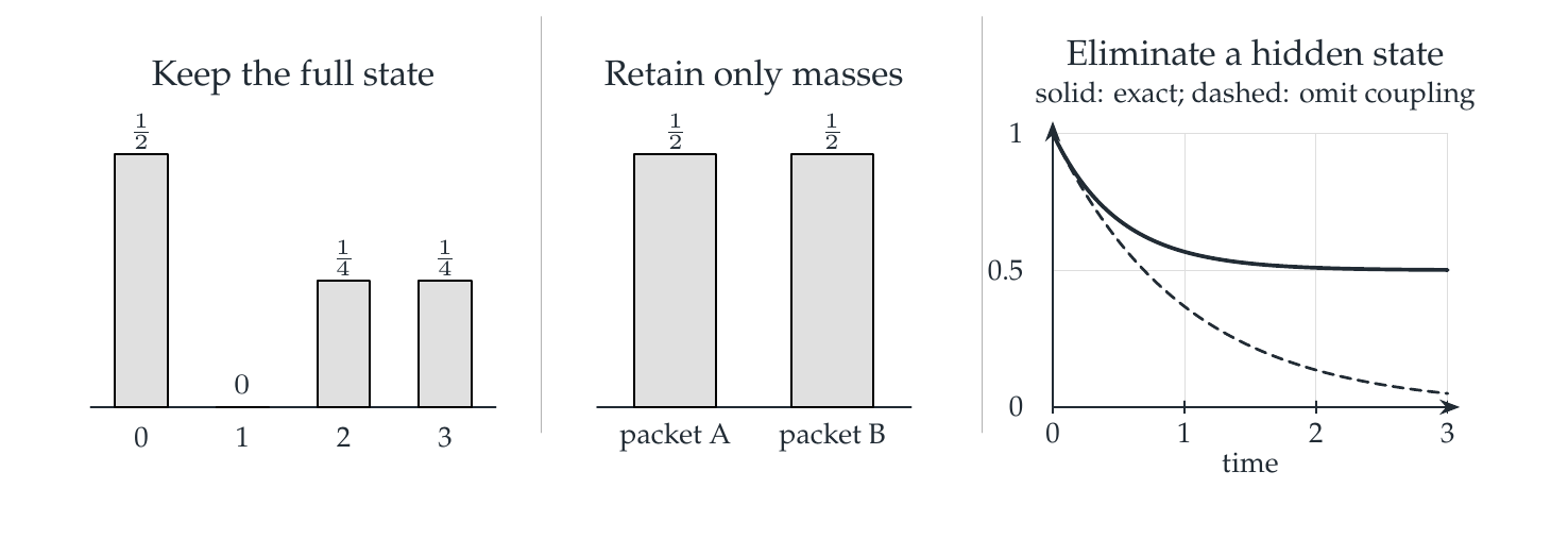
Read left to right. The first two panels use the same distribution: the middle panel sums states into two packets and loses the within-packet shape. The separate right-hand model compares the exact retained evolution with the result of omitting its coupling. The solid and dashed curves start together and then separate. The curve panel is a different model from the bars.
Drawing labels and data 24 labels
Read the original labels as selectable text. Tables preserve grid relationships; other short labels are grouped compactly.
| State | Probability |
|---|---|
| 0 | \(\frac{1}{2}\) |
| 1 | \(0\) |
| 2 | \(\frac{1}{4}\) |
| 3 | \(\frac{1}{4}\) |
| Packet | Mass |
|---|---|
| packet A | \(\frac{1}{2}\) |
| packet B | \(\frac{1}{2}\) |
Retained and hidden states
- Eliminate a hidden state
- solid: exact; dashed: omit coupling
Horizontal axis and ticks
time, 0, 1, 2, 3
Vertical ticks
0, 0.5, 1
Evidence note from the source edition
Left and center use one probability vector and its two block masses. The right panel is a separate retained/hidden model, developed on Visual 22. Every curve is drawn from an explicit formula.
Coordinates retain; aggregation forgets; elimination remembers
Keeping every component \(P_a x\) is an exact change of representation when \(\sum_aP_a=I\). Reconstruct by summing the components. In contrast, replacing \((p_0,p_1,p_2,p_3)\) by \((p_0+p_1,p_2+p_3)\) forgets how mass was distributed inside either pair. That information can matter for later observations.
Eliminating a hidden state is different again. Its coordinates disappear from the displayed state, but the exact retained equation acquires a history integral. Simply deleting the coupling produces the dashed curve above, not the original evolution.
| Question | Worked route | Pages |
|---|---|---|
| When is coarse evolution exact? | Aggregate columns, then test intertwining. | Visual 4–Visual 6 |
| When is a coarse posterior exact? | Compare two hidden shapes with the same masses. | Visual 9–Visual 13 |
| What changes under a fractional power? | Keep modes, change spectral rates. | Visual 15–Visual 17 |
| What returns after elimination? | Compute the self-energy and memory kernel. | Visual 21–Visual 25 |
Read this as
The paper supplies exact identities and conditional bounds. Whether a particular coarse model satisfies their hypotheses is a separate calculation.