
The function \(a\mapsto\sqrt a\) changes most rapidly near zero. A scalar model already shows why a spectral gap appears in fractional-defect estimates:
The same input difference has a square-root scale at zero and a linear bound above a fixed positive lower bound.
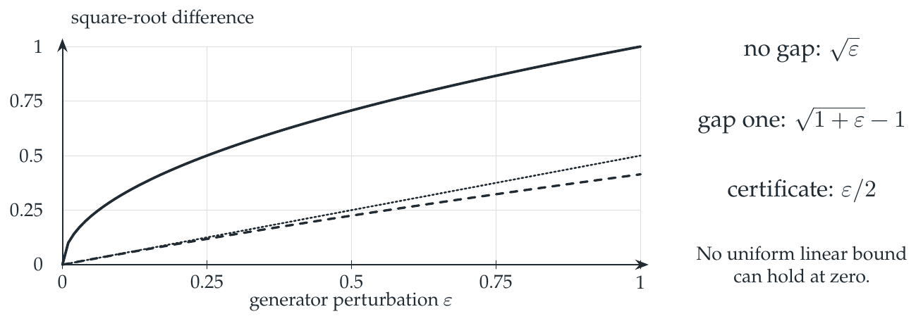
Reading the drawing
The horizontal axis is generator perturbation. The upper curve is the ungapped difference; the lower curve is the gapped difference. A straight certificate is shown alongside the gapped case, and the note states the limitation at zero.
Drawing labels and data 16 labels
Read the original labels as selectable text. Tables preserve grid relationships; other short labels are grouped compactly.
- 0
- 0.25
- 0.5
- 0.75
- 1
- 0
- 0.25
- 0.5
- 0.75
- 1
- generator perturbation \(\varepsilon\)
- square-root difference
- no gap: \(\sqrt{\varepsilon}\)
- gap one: \(\sqrt{1+\varepsilon}-1\)
- certificate: \(\varepsilon/2\)
No uniform linear bound
can hold at zero.
Evidence note from the source edition
The upper curve compares \(0\) with \(\varepsilon\). The lower curve compares \(1\) with \(1+\varepsilon\). The dotted line \(\varepsilon/2\) bounds the latter. All plotted values come from the displayed scalar formulas.
Read an operator bound with its hypotheses
For positive self-adjoint finite matrices \(A,B\ge mI\) and \(0<\alpha<1\), the manuscript's gapped estimate has the form
It concerns an intertwining defect, not just two eigenvalue lists. With \(C=1\), \(A=4\), \(B=9\), \(m=4\), and \(\alpha=1/2\), the generator defect has size \(5\), the fractional defect has size \(1\), and the bound is \(5/4\).
The common zero mode of a Markov generator cannot simply be included in a positive-gap estimate. One must either work on an appropriate gapped subspace, handle the zero mode separately, or use the gapless estimate. In particular, a good estimate on each finite level need not have a constant uniform in the refinement level.
On Visual 27, the sequences \(1/n^2\) and \(1/n\) turn this change in error scale into a concrete distinction between summable and nonsummable defects.
Read this as
A fixed gap is quantitative information. It prevents the derivative of the fractional function from becoming singular along the comparison.