
For a small exact example, take the \(\mathrm{Beta}(2,3)\) density
Observe a specified ordered sequence with two successes and one failure. Its likelihood is \(\theta^2(1-\theta)\). Multiplication adds exponents, so the posterior belongs to \(\mathrm{Beta}(4,4)\) with density \(140\theta^3(1-\theta)^3\).
Reading the drawing
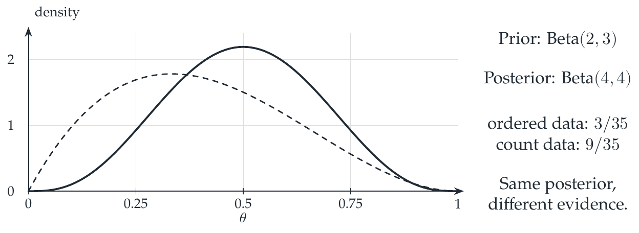
The dashed curve is the prior and the solid curve is the posterior after the stated observation. The right-hand notes distinguish the evidence for ordered data from the evidence for count data, while retaining the same posterior.
Drawing labels and data 14 labels
Read the original labels as selectable text. Tables preserve grid relationships; other short labels are grouped compactly.
- 0
- 0.25
- 0.5
- 0.75
- 1
- 0
- 1
- 2
- \(\theta\)
- density
Prior: \(\mathrm{Beta}(2,3)\)
Posterior: \(\mathrm{Beta}(4,4)\)
ordered data: \(3/35\)
count data: \(9/35\)
Same posterior,
different evidence.
Evidence note from the source edition
The dashed prior is asymmetric. The solid posterior is symmetric with mean \(1/2\). Polynomial integration verifies the normalizers exactly; the curves are sampled drawings of those polynomials.
The observation convention changes the evidence
The integral of the unnormalized posterior is
Dividing by \(3/35\) gives the displayed normalized density. If the observation is instead the count of two successes in three trials, there are \(\binom32=3\) compatible ordered sequences. The count likelihood is therefore \(3\theta^2(1-\theta)\) and its evidence is \(9/35\).
The extra factor does not depend on \(\theta\), so it cancels from the posterior. The two experiments thus have the same posterior distribution but different data probabilities. Evidence is not determined by the final normalized density alone.
The exact check also integrates both densities to one and integrates \(\theta\) against the posterior to obtain \(1/2\). This demonstrates one conjugate family in elementary terms. It does not show that arbitrary likelihoods preserve that family or that all posterior information can be compressed into two exponents.
Read this as
Conjugacy gives a closed parameter update when a specified likelihood respects a specified family. Preserve the evidence as well as the normalized posterior.