
Group states \(0,1\) into A and states \(2,3\) into B. The aggregation map and the candidate coarse kernel are
A fine state in A has probability \(1/4\) of entering B in one step, regardless of which fine state in A was occupied. The analogous statement holds for B.
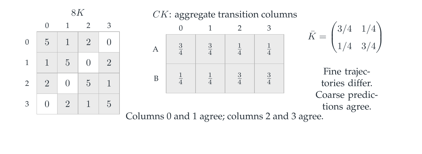
Reading the drawing
The left table is eight times the fine transition matrix, with target states as rows and source states as columns. The middle table sums target rows into packets A and B. Its first two columns agree, as do its last two. The right-hand coarse matrix and the original comparison note follow the tables.
Drawing labels and data 43 labels
Read the original labels as selectable text. Tables preserve grid relationships; other short labels are grouped compactly.
| Target / source | 0 | 1 | 2 | 3 |
|---|---|---|---|---|
| 0 | \(5\) | \(1\) | \(2\) | \(0\) |
| 1 | \(1\) | \(5\) | \(0\) | \(2\) |
| 2 | \(2\) | \(0\) | \(5\) | \(1\) |
| 3 | \(0\) | \(2\) | \(1\) | \(5\) |
| Coarse packet / fine source | 0 | 1 | 2 | 3 |
|---|---|---|---|---|
| A | \(\frac{3}{4}\) | \(\frac{3}{4}\) | \(\frac{1}{4}\) | \(\frac{1}{4}\) |
| B | \(\frac{1}{4}\) | \(\frac{1}{4}\) | \(\frac{3}{4}\) | \(\frac{3}{4}\) |
- Columns 0 and 1 agree; columns 2 and 3 agree.
Fine trajectories differ.
Coarse predictions agree.
Evidence note from the source edition
The fine columns are visibly different. Their sums over each target packet agree within each source packet. That equality is the reason a two-state description works.
A one-step calculation controls every discrete horizon
The displayed columns give \(CK=\bar KC\). Multiplication then yields
For example, \(e_0\) and \(e_1\) have the same coarse initial vector \((1,0)^{\mathsf T}\). Their fine evolutions differ, but their coarse vectors agree at every step. No choice of the within-A conditional distribution is needed for the prediction.
The continuous generator also closes:
The Duhamel identity therefore gives \(Ce^{tQ}=e^{t\bar Q}C\). This is a second consequence of the corresponding generator identity, not an inference that \(K\) is a fixed-time sample of \(Q\).
Aggregation is still not invertible. The theorem says the discarded details are irrelevant for these predictions. It does not say they are irrelevant to every later likelihood. The observation counterexample on Visual 10 uses this exact same partition.
Read this as
A partition is not automatically a valid Markov model. The aggregate transition columns must be constant within each source block.