
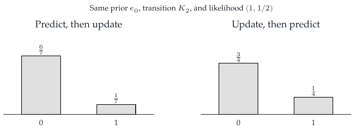
Use the two-state kernel \(K_2\) from Visual 2, the initial distribution \(e_0\), and likelihood \((1,1/2)\). Predicting first gives \((3/4,1/4)\). Its likelihood-weighted vector is \((3/4,1/8)\), with evidence \(7/8\), so the posterior is \((6/7,1/7)\).
Updating first leaves \(e_0\) unchanged. Predicting afterward gives \((3/4,1/4)\) instead. The order of operations expresses which time the observation concerns.
Reading the drawing
Both panels start from the same prior, transition, and likelihood, as stated above them. The displayed probability vectors differ. The left panel uses prediction first; the right panel applies the observation first.
Drawing labels and data 11 labels
Read the original labels as selectable text. Tables preserve grid relationships; other short labels are grouped compactly.
- Predict, then update
- 0
\(\frac{6}{7}\)
- 1
\(\frac{1}{7}\)
- Update, then predict
- 0
\(\frac{3}{4}\)
- 1
\(\frac{1}{4}\)
Same prior \(e_0\), transition \(K_2\), and likelihood \((1,1/2)\)
Evidence note from the source edition
Both routes produce valid probability vectors. Their difference is therefore not a normalization bug. It is a different conditioning problem.
Keep an unnormalized path alongside the filter
For a sequence of observations, let \(D_r={\operatorname{diag}}(\lambda^{(r)})\). The forward recursion is
Its unnormalized companion is
The product of evidences records the normalization lost at each individual step. The four-state computation on Visual 26 checks both paths independently, including their coarse versions.
Here \(D_rK\) means an observation after prediction. In the Feynman–Kac example on Visual 20, departure-state weighting has forward operator \(K D_w\). Both conventions are legitimate once their meanings are fixed, but they cannot be substituted for one another.
Read this as
Write the chronological sequence before multiplying matrices. A product can be normalized correctly and still answer the wrong time-ordered question.