
For a prior \(p\), let \(P=Cp\) and let \(r_a(p)\) be the conditional average of the fine likelihood inside packet \(a\). For the uniform prior and \(\lambda=(4,1,1,1)\),
The exact coarse posterior is \(\mathcal B_r(P)=(5/7,2/7)^{\mathsf T}\). Suppose instead that the declared coarse likelihood is \(\bar\lambda=(1,1)\).
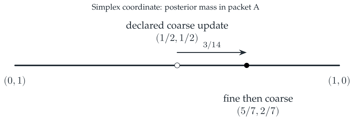
Reading the drawing
The line represents posterior mass in the first packet. An open point marks the declared coarse update and a filled point marks updating first in the fine model. The arrow gives their displayed difference.
Drawing labels and data 6 labels
Read the original labels as selectable text. Tables preserve grid relationships; other short labels are grouped compactly.
- \((0,1)\)
- \((1,0)\)
declared coarse update
\((1/2,1/2)\)
fine then coarse
\((5/7,2/7)\)
- \(3/14\)
- Simplex coordinate: posterior mass in packet A
Evidence note from the source edition
The posterior error lies along the mass-preserving direction of the two-state simplex. Its entries are opposite because both endpoints have total mass one.
Compute the factorization, including the null direction
Here \(\bar b=\mathcal B_{\bar\lambda}(P)=P\), \(\delta=r-\bar\lambda=(3/2,0)^{\mathsf T}\), and \(Z_r=7/4\). Hence
This is the actual fine-to-coarse discrepancy, not a fitted approximation. The matrix kills \(\bar\lambda\), recording the common-scale null direction. Its \(\ell^1\) error is \(3/7\).
For a family of likelihoods, states may be grouped by equality of their whole likelihood profile. The family \((3,3,1,1)\) and \((1,2,1,2)\) separates all four states even though either likelihood alone permits a coarser grouping. The common refinement is therefore the discrete partition. The theorem's one-packet exception still remains.
Read this as
The defect factors through exactly the conditional evidence information missing from the declared coarse model. A new observation family can require a finer partition.