
Take three interior nodes \(x_i=i/4\) on \([0,1]\), with zero boundary values and \(h=1/4\). The discrete negative second derivative is
For the continuous Dirichlet problem, the Green function is \(G(x,y)=\min(x,y)-xy\). At these nodes the exact comparison is
Reading the drawing
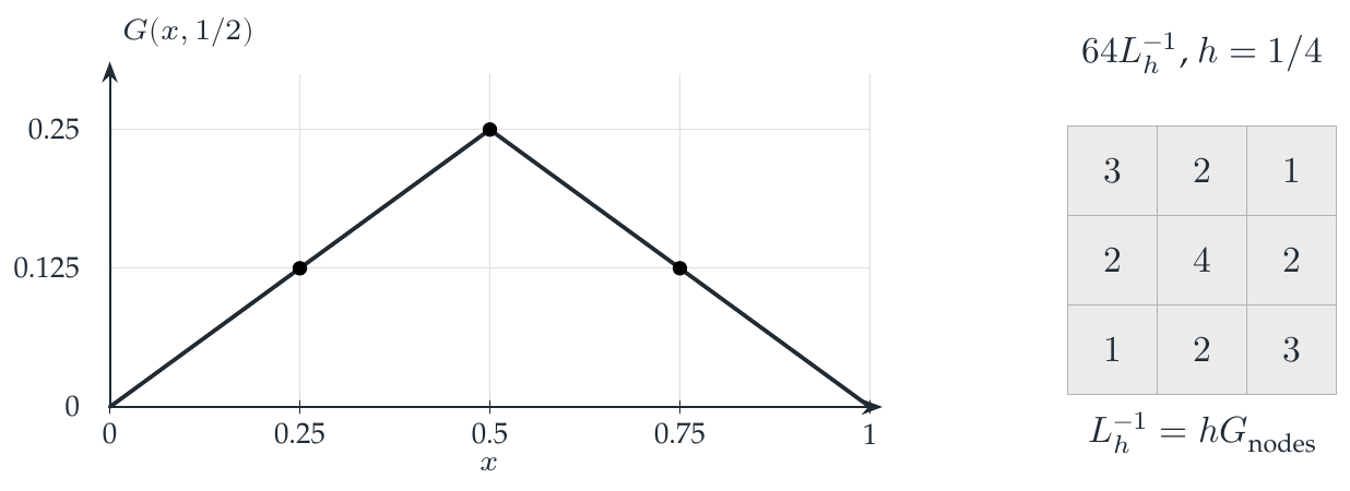
The left graph samples one Green-function column at grid nodes. The matrix at right is the displayed scaled finite inverse. The equation beneath it keeps the grid-spacing factor between the nodal Green values and the inverse operator.
Drawing labels and data 21 labels
Read the original labels as selectable text. Tables preserve grid relationships; other short labels are grouped compactly.
- 0
- 0.25
- 0.5
- 0.75
- 1
- 0
- 0.125
- 0.25
- \(x\)
- \(G(x,1/2)\)
- \(64 L_h^{-1}\), \(h=1/4\)
| Row / column | Column 1 | Column 2 | Column 3 |
|---|---|---|---|
| Row 1 | \(3\) | \(2\) | \(1\) |
| Row 2 | \(2\) | \(4\) | \(2\) |
| Row 3 | \(1\) | \(2\) | \(3\) |
- \(L_h^{-1}=hG_{\rm nodes}\)
Evidence note from the source edition
The tent is the central column of the continuous Green kernel. It has nodal values \((1,2,1)/8\); its discrete inverse column is \((1,2,1)/32\), smaller by the factor \(h\).
A forcing vector is not a quadrature-weighted measure
For sampled forcing \(f_j\), the finite solution is
The factor \(h\) converts samples into the quadrature weights appropriate to this formula. Dropping it multiplies the computed solution by four on the displayed grid.
A discrete unit coordinate vector and a discretized unit point mass use different normalizations. For \(f=e_2\), the result is the second inverse column. For \(f=e_2/h\), it is the unscaled tent sampled at the nodes. Either convention can be useful, but it must be specified before comparing answers.
Exact checks multiply \(L_h\) by the proposed inverse at \(1,3,7,\) and \(15\) interior nodes. The general identity is the manuscript theorem. These finite checks do not extend it to arbitrary meshes, dimensions, or boundary conditions.
Read this as
An inverse kernel carries a measure convention. A correct-looking tent can give a wrong solution if the grid weight is omitted.