Paper VI visual guide · Visual 10 of 42 · SUFFICIENCY / A COMPUTABLE FAILURE WITNESS

Two priors that fool the coarse model

Traditional Part I: Theorem 8.2 and the one-packet exception.

Keep the same likelihood \(\lambda=(4,1,1,1)^{\mathsf T}\) and partition A\(=\{0,1\}\), B\(=\{2,3\}\). Compare

\[ p^{(a)}=(1/2,0,1/2,0)^{\mathsf T},\qquad p^{(b)}=(0,1/2,1/2,0)^{\mathsf T}. \]

Both have coarse prior \((1/2,1/2)^{\mathsf T}\). A procedure given only that two-entry vector cannot distinguish them.

Two priors with the same coarse masses produce different coarse posteriors. — Original drawing. Read the description below; expand the labels and data for selectable text.

Reading the drawing

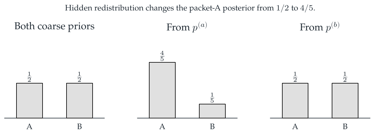
The left panel gives their common two-packet prior. The middle and right panels give the two updated packet distributions. The note above attributes the difference to redistribution hidden inside the first packet.

Drawing labels and data 16 labels

Read the original labels as selectable text. Tables preserve grid relationships; other short labels are grouped compactly.

Both coarse priors
A

\(\frac{1}{2}\)

From \(p^{(a)}\)
A

\(\frac{4}{5}\)

\(\frac{1}{5}\)

From \(p^{(b)}\)
A

\(\frac{1}{2}\)

Hidden redistribution changes the packet-A posterior from \(1/2\) to \(4/5\).

Open the full-size drawing

Drawing source with line numbers

Evidence note from the source edition

After the identical fine likelihood is applied, the coarse posteriors are \((4/5,1/5)\) and \((1/2,1/2)\). A single deterministic update of the common coarse prior cannot produce both.

Permalink · Source line 222

Why this witnesses the necessity of blockwise constancy

Permalink · Source line 223

The A evidence for \(p^{(a)}\) is \(2\), whereas it is \(1/2\) for \(p^{(b)}\). Their B evidence is \(1/2\) in both cases. The posterior odds therefore distinguish the hidden distribution inside A.

For strictly positive fine and coarse likelihoods, and at least two coarse blocks, the manuscript proves the all-prior criterion

\[ C\mathcal B_\lambda(p)=\mathcal B_{\bar\lambda}(Cp)\quad\hbox{for every }p \quad\Longleftrightarrow\quad \lambda_i=c\bar\lambda_a\quad(i\in I_a) \]

for one global \(c>0\). The global scale is invisible after normalization. A different arbitrary scale for each packet is not invisible: it changes posterior odds.

If all states are merged into a single packet, every normalized posterior coarsens to \((1)\). That degenerate commutation holds for every likelihood and cannot identify any within-packet information. It is explicitly excluded from the nontrivial criterion.

Permalink · Source line 224

Read this as

A prior-dependent effective likelihood can always summarize the update. A fixed likelihood that works for every prior is a much stronger requirement.

Permalink · Source line 235

Source and conversion record

The original atlas wording, equations, and drawing labels are retained. Drawings are views of the frozen visual-guide PDF. Text descriptions and table headings are added reading aids. This conversion does not rebuild TeX, rerun the examples, audit proofs or compile Lean.

Conversion checks and source hashes