Paper VI: Exact Bayesian refinement and information-loss packets

8 Exact Bayesian refinement and information-loss packets

On this page · Visual guide: Three ways to reduce a model · Permalink · Source line 827

How to read the result

The all-prior criterion here tests coarse posterior masses for every prior and assumes at least two coarse blocks. Part II uses a stronger convention that also preserves each conditional distribution inside a block. These are different contracts, so the one-block boundary must be read with its own definition.

Permalink · Source line 828

Two rational priors with the same two coarse masses. A blockwise constant likelihood gives the same coarse update, while a likelihood varying within a block separates the posteriors. The exact fractions are calculated before plotting.

Let the fine state set \(I\) be partitioned into nonempty coarse packets \(I_a\), \(a\in A\). The coarsening map on probability vectors is

\[ (C_\pi p)_a=P_a=\sum_{i\in I_a}p_i. \]

For a fine likelihood \(\lambda=(\lambda_i)_{i\in I}\) and a prior \(p\), define the effective coarse likelihood

\[ r_a(p) = \frac{\sum_{i\in I_a}\lambda_i p_i}{P_a} \qquad(P_a>0). \]

Its value on a zero-mass packet is irrelevant and may be set to zero.

Permalink · Source line 839

Theorem 8.1: Exact effective-likelihood factorization

Whenever the fine evidence is positive,

\[ \boxed{ C_\pi{\mathcal B}_\lambda(p) = {\mathcal B}_{r(p)}(C_\pi p).} \]

Thus the only fine information needed for the coarse posterior, beyond the coarse prior masses, is the vector of conditional packet evidences \(r(p)\).

Read proof · Visual guide: The exact information-loss vector · Read statement and proof side by side · Permalink · Source line 852 · Claim record · Lean coverage · Code · Worked examples

Proof of Theorem 8.1

For \(P=C_\pi p\) and \(Z=\sum_i\lambda_ip_i=\sum_aP_ar_a(p)\),

\[ \bigl(C_\pi{\mathcal B}_\lambda(p)\bigr)_a = \frac{\sum_{i\in I_a}\lambda_ip_i}{Z} = \frac{P_ar_a(p)}{\sum_bP_br_b(p)} = \bigl({\mathcal B}_{r(p)}(P)\bigr)_a. \]

Back to statement · Read statement and proof side by side · Permalink · Source line 863 · Claim record · Lean coverage · Code · Worked examples

The next result gives the exact necessary and sufficient condition for a coarse likelihood to work for every prior.

Permalink · Source line 876

Theorem 8.2: Bayesian refinement criterion

Assume that the partition contains at least two coarse packets and that the fine and coarse likelihoods are strictly positive. The identity

\[ \boxed{ C_\pi{\mathcal B}_\lambda(p) = {\mathcal B}_{\bar\lambda}(C_\pi p)} \]

holds for every fine prior \(p\) if and only if there exists one scalar \(c>0\) such that

\[ \boxed{ \lambda_i=c\,\bar\lambda_a \qquad(i\in I_a).} \]

Equivalently, the likelihood is constant on each coarse packet, with the coarse values determined up to the globally invisible Bayesian scaling \(c\).

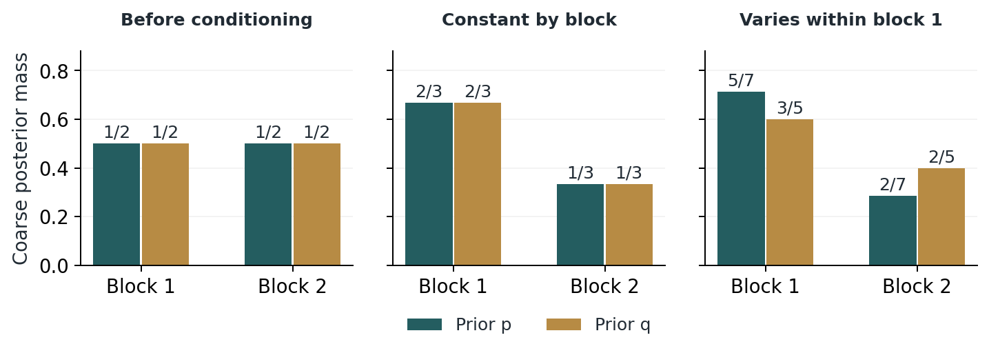
Read proof · Visual guide: Two priors that fool the coarse model · Visual guide: One complete coarse filter · Read statement and proof side by side · Permalink · Source line 878 · Claim record · Lean coverage · Code · Worked examples

Proof of Theorem 8.2

If \(\lambda_i=c\bar\lambda_a\) on \(I_a\), then \(P_a r_a(p)=c\bar\lambda_aP_a\) for every prior, including zero-mass packets, and the preceding theorem gives the desired identity because Bayesian normalization removes the common scalar \(c\).

Conversely, fix two fine states \(i,i'\in I_a\) and one state \(j\in I_b\) in another coarse packet. Vary the distribution of a fixed coarse mass inside \(I_a\) between \(i\) and \(i'\) while leaving every coarse packet mass unchanged. The right side depends only on those coarse masses and is therefore unchanged. The left-side posterior mass of packet \(a\) depends on the conditional average of \(\lambda_i\) and \(\lambda_{i'}\). It can be independent of that variation only if \(\lambda_i=\lambda_{i'}\). Hence \(\lambda\) is constant on every packet; write the value on \(I_a\) as \(\lambda_a\).

Now use priors supported on one state of packet \(a\) and one state of packet \(b\). Equality of the two coarse posterior odds gives

\[ \frac{\lambda_a}{\lambda_b} = \frac{\bar\lambda_a}{\bar\lambda_b}. \]

This holds for every pair of coarse packets, so \(\lambda_a=c\bar\lambda_a\) for one common \(c>0\).

Back to statement · Read statement and proof side by side · Permalink · Source line 895 · Claim record · Lean coverage · Code · Worked examples

Remark 8.3: The one-packet boundary

If the coarse partition has only one packet, every posterior coarsens to the scalar \(1\), so commutation is automatic and no within-packet likelihood information can be identified. The nontrivial criterion begins with at least two coarse packets.

Permalink · Source line 909

When sufficiency fails, the defect still has an exact finite factorization. Fix a declared coarse likelihood \(\bar\lambda\), put

\[ P=C_\pi p, \qquad \delta(p)=r(p)-\bar\lambda, \qquad \bar b={\mathcal B}_{\bar\lambda}(P), \qquad Z_r=\langle r(p),P\rangle. \]

Permalink · Source line 913

Theorem 8.4: Bayesian information-loss packet

Assume nonnegative fine and declared coarse likelihoods, with both \(Z_r>0\) and \(Z_{\bar\lambda}>0\). The coarsening defect is

\[ \boxed{ C_\pi{\mathcal B}_\lambda(p) - {\mathcal B}_{\bar\lambda}(P) = \frac{1}{Z_r} \left({\operatorname{diag}}(P)-\bar bP^{\mathsf T}\right) \delta(p).} \]

The factor matrix annihilates \(\bar\lambda\). This records the common-scale null direction at the declared coarse likelihood; the full exact defect remains homogeneous under simultaneous likelihood rescaling because the numerator and evidence denominator scale together. Moreover,

\[ \boxed{ \left\|C_\pi{\mathcal B}_\lambda(p)-{\mathcal B}_{\bar\lambda}(P)\right\|_1 \le \frac{2\sum_aP_a|\delta_a(p)|} {\min\{Z_r,Z_{\bar\lambda}\}}} \]

and

\[ \sum_aP_a|\delta_a(p)| \le \sum_i p_i\left|\lambda_i-\bar\lambda_{\pi(i)}\right|. \]

Read proof · Visual guide: The exact information-loss vector · Read statement and proof side by side · Permalink · Source line 924 · Claim record · Lean coverage · Code · Worked examples

Proof of Theorem 8.4

The effective-likelihood theorem reduces the defect to

\[ {\mathcal B}_{\bar\lambda+\delta}(P)-{\mathcal B}_{\bar\lambda}(P). \]

Since \(Z_r=Z_{\bar\lambda}+P^{\mathsf T}\delta\), direct subtraction gives

\[ \frac{1}{Z_r} \left({\operatorname{diag}}(P)-\bar bP^{\mathsf T}\right)\delta. \]

Also,

\[ \left({\operatorname{diag}}(P)-\bar bP^{\mathsf T}\right)\bar\lambda =P\odot\bar\lambda-\bar bZ_{\bar\lambda}=0. \]

The first norm bound is the likelihood perturbation theorem applied on the coarse simplex. For a zero-mass packet, both sides of the following estimate vanish. For \(P_a>0\),

\[ P_a|\delta_a| = P_a\left|\sum_{i\in I_a}\frac{p_i}{P_a} (\lambda_i-\bar\lambda_a)\right| \le \sum_{i\in I_a}p_i|\lambda_i-\bar\lambda_a|, \]

and summing over \(a\) proves the second inequality.

Back to statement · Read statement and proof side by side · Permalink · Source line 952 · Claim record · Lean coverage · Code · Worked examples

Corollary 8.5: Nested Bayesian packet tower

Consider a nested finite packet tower with strictly positive likelihoods at every level. At each adjacent coarsening with at least two coarse packets, commutation for every prior is equivalent to the fine likelihood being blockwise proportional to the declared coarse likelihood, with one common positive proportionality factor. An adjacent coarsening to a single packet commutes automatically and imposes no such condition. Under these conditions, all composite coarsening squares commute.

Read proof · Read statement and proof side by side · Permalink · Source line 979 · Claim record · Lean coverage · Code · Worked examples

Proof of Corollary 8.5

At each adjacent coarsening with at least two coarse packets, apply the refinement criterion. For a single coarse packet, both normalized posteriors equal 1. Composition of these commuting squares gives the full tower statement.

Back to statement · Read statement and proof side by side · Permalink · Source line 983 · Claim record · Lean coverage · Code · Worked examples

Corollary 8.6: Canonical coarsest likelihood-resolving partition

For a finite family of likelihoods \(\{\lambda^{(y)}\}_{y\in Y}\), define

\[ i\sim j \quad\Longleftrightarrow\quad \lambda_i^{(y)}=\lambda_j^{(y)} \text{ for every }y\in Y. \]

The equivalence classes form the unique coarsest likelihood-resolving partition: every likelihood is constant on each packet. Every update therefore closes on this partition whenever its evidence is positive. If all likelihoods are strictly positive and there are at least two profile classes, this is also the unique coarsest nontrivial partition on which every update closes for every prior. The one-packet partition always closes, independently of the profiles, and is excluded from this last assertion.

Read proof · Visual guide: The exact information-loss vector · Read statement and proof side by side · Permalink · Source line 987 · Claim record · Lean coverage · Code · Worked examples

Proof of Corollary 8.6

Equality of likelihood profiles is an equivalence relation. Its classes are likelihood-resolving by definition, and every likelihood-resolving partition refines them. Exact closure follows by summing the weighted masses in each fiber, including zero-mass fibers. Under strict positivity, the refinement criterion implies that every nontrivial all-prior closed partition is likelihood-resolving. When every profile is identical, all partitions close; there need not be a unique coarsest nontrivial partition.

Back to statement · Read statement and proof side by side · Permalink · Source line 998 · Claim record · Lean coverage · Code · Worked examples

For strictly positive likelihoods and at least two coarse packets, the Bayesian refinement square commutes for every prior exactly when the likelihood is constant on each coarsening fiber, up to one global scale.

When packet sufficiency fails, the exact defect factors through the difference between the conditional effective likelihood and the declared coarse likelihood.

Numerical certificate 8.7: Bayesian refinement

For the finite test partition \(\{0,1\}\sqcup\{2,3\}\), a blockwise-constant likelihood gave commutation residual \(1.11\times10^{-16}\). A nonconstant likelihood produced an exact defect-factorization residual \(7.29\times10^{-17}\). Its measured \(L^1\) defect was \(4.8787\times10^{-2}\), below the certified bound \(1.1016\times10^{-1}\). Two priors with identical coarse masses but different hidden within-packet shapes produced coarse posteriors differing by \(1.2400\times10^{-1}\), which is a direct necessity witness.

Permalink · Source line 1016 · Claim record · Lean coverage · Code · Worked examples

Boundary 8.8: Finite exact theorem

The conjectured Bayesian refinement law is therefore resolved for finite packet systems and arbitrary priors. Infinite-dimensional disintegration, posterior consistency, and stability of data-dependent partitions require their own measure-theoretic and asymptotic hypotheses.

Permalink · Source line 1020 · Claim record · Lean coverage · Code · Worked examples

Source and conversion record

Source SHA-256: 736e615131f57daf341b6cb0600761d58950450947c85d433206148cca228333

Unsupported prose commands stop the build. The mathematical expression sequence is checked against the source, with manuscript macros expanded for display.

Conversion records

Read and explore

Proofs and implementation

About this work

Other resources