
Keep the weights and observable from Visual 7. Let \(E_0f\) be the constant global mean, let \(E_1=E\) average within A and B, and let \(E_2=I\) retain every value. Define
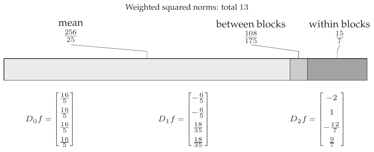
Then \(D_0f\) is the mean, \(D_1f\) describes the contrast between block means, and \(D_2f\) is the fluctuation left inside each block.
Reading the drawing
Three adjacent segments represent the displayed orthogonal contributions. Their values appear above the bar, and the three component vectors appear below it. The source plate identifies the weighted inner product used for this decomposition.
Drawing labels and data 7 labels
Read the original labels as selectable text. Tables preserve grid relationships; other short labels are grouped compactly.
mean
\(\frac{256}{25}\)
between blocks
\(\frac{108}{175}\)
within blocks
\(\frac{15}{7}\)
- Weighted squared norms: total \(13\)
Evidence note from the source edition
The strip lengths are proportional to the three exact weighted energies. The between-block component is small but not zero. The vectors below specify the corresponding directions, not only their sizes.
The energy identity follows from actual orthogonality
The tower identities give \(E_0E_1=E_1E_0=E_0\). Together with weighted self-adjointness, these imply
For the chosen \(f\), the total weighted energy is \(\|f\|_\pi^2=13\) and the mean is \(16/5\). Consequently
The first term is the energy of the between-block contrast, and the second is the weighted within-block variance. This is a decomposition of one observable in one fixed weighted space.
Changing the probability weights between levels would change the inner products and the averaging operators. The displayed orthogonal decomposition would no longer follow merely from nesting the sets. Likewise, choosing unrelated projections can preserve the telescope \(\sum D_j=I\) while losing orthogonality and the energy sum.
Read this as
The differences between nested conditional expectations are not just bookkeeping. They are orthogonal, separately measurable parts of the original signal.