
Return to the four-state generator on Visual 4 and put \(L=-Q\). It is real symmetric and nonnegative, with orthogonal projectors \(P_0,P_1,P_2,P_3\) and eigenvalues \(0,2,4,6\). Its square root is
Both heat evolutions retain these modes. Ordinary diffusion multiplies mode \(j\) by \(e^{-2jt}\); square-root diffusion multiplies it by \(e^{-\sqrt{2j}\,t}\). The constant mode is unchanged in both.
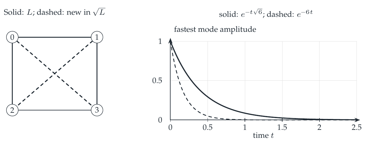
Reading the drawing
The left graph distinguishes the original couplings from the added fractional couplings. The right plot compares the two displayed decay factors for the fastest mode. The source retains the same spectral modes while changing their clocks.
Drawing labels and data 17 labels
Read the original labels as selectable text. Tables preserve grid relationships; other short labels are grouped compactly.
- 0
- 1
- 2
- 3
- Solid: \(L\); dashed: new in \(\sqrt L\)
- 0
- 0.5
- 1
- 1.5
- 2
- 2.5
- 0
- 0.5
- 1
- time \(t\)
- fastest mode amplitude
- solid: \(e^{-t\sqrt6}\); dashed: \(e^{-6t}\)
Evidence note from the source edition
The highest mode decays at rates \(6\) and \(\sqrt6\). The graph beside the curves shows the additional couplings in the fractional operator. Curves display the explicit formulas, not an empirical fit.
Fractional does not mean entrywise
Although \(L_{03}=0\), its spectral square root satisfies
Thus \(-L^{1/2}\) permits a direct transition between states \(0\) and \(3\), which were not neighbors for \(Q\). Taking the square root of each matrix entry would neither produce this value nor square back to \(L\).
The exact block aggregation remains compatible in this example:
The coarse matrix is the positive square root of \(-Q_c\). This is a concrete naturality identity, checked on the full matrices. It is not a claim that an arbitrary partition commutes with every fractional construction.
The computation uses a nonnegative self-adjoint operator and a specified spectral branch. General nonnormal matrices, unbounded domains, and positivity of other fractional evolutions need their own hypotheses.
Read this as
Fractional powers alter modal decay rates. Reassembling those modes can introduce long-range spatial interactions even when the original generator was sparse.