
A packet calculus can reorganize a signal exactly, choose among finitely many representations, or describe a nonlinear coordinate geometry. These are not the same task. This guide keeps one concrete object in view for each, so that the reader can compute rather than only follow arrows.
Reading the drawing
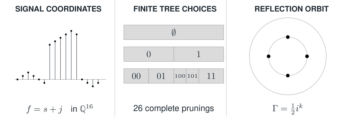
Three panels compare the sample signal, a finite binary tree and a reflection orbit. The panels illustrate separate coordinate, selection and nonlinear questions.
Drawing labels and data 14 labels
Read the original labels as selectable text. Tables preserve grid relationships; other short labels are grouped compactly.
- SIGNAL COORDINATES
- FINITE TREE CHOICES
- REFLECTION ORBIT
- \(f=s+j\quad\text{in }{\mathbb Q}^{16}\)
- \(\varnothing\)
- \(0\)
- \(1\)
- \(00\)
- \(01\)
- \(100\)
- \(101\)
- \(11\)
- 26 complete prunings
- \(\Gamma=\tfrac12 i^k\)
A signal that can be checked by hand
Our main finite signal is \(f=s+j\in{\mathbb Q}^{16}\). The background repeats
and \(j[n]=3\) at \(6\le n<12\), with \(j[n]=0\) elsewhere. This is a discrete background model, not an assertion of continuum smoothness. Its energy is exactly \(57\). We use it for residue coordinates, Haar transforms, coefficient deletion, and known-packet cancellation.
A tree whose alternatives can all be seen
The full binary tree of depth three has only \(26\) complete prunings. We enumerate all of them, compute a unique mixed-depth optimum, and certify its stability with rational costs. The displayed objective is deliberately explicit, not claimed to be a universal signal-quality score.
A coordinate orbit with no hidden numerical poles
The four reflection points \(\Gamma=i^k/2\) map to four exact impedances. A second orbit passes through infinity; homogeneous coordinates make that point an ordinary part of the construction.
Read this as
Exact coordinates preserve information. An optimizer chooses coordinates. An estimator must still identify information not already supplied.