
Away from \(\Gamma=1\), the inverse Cayley map satisfies
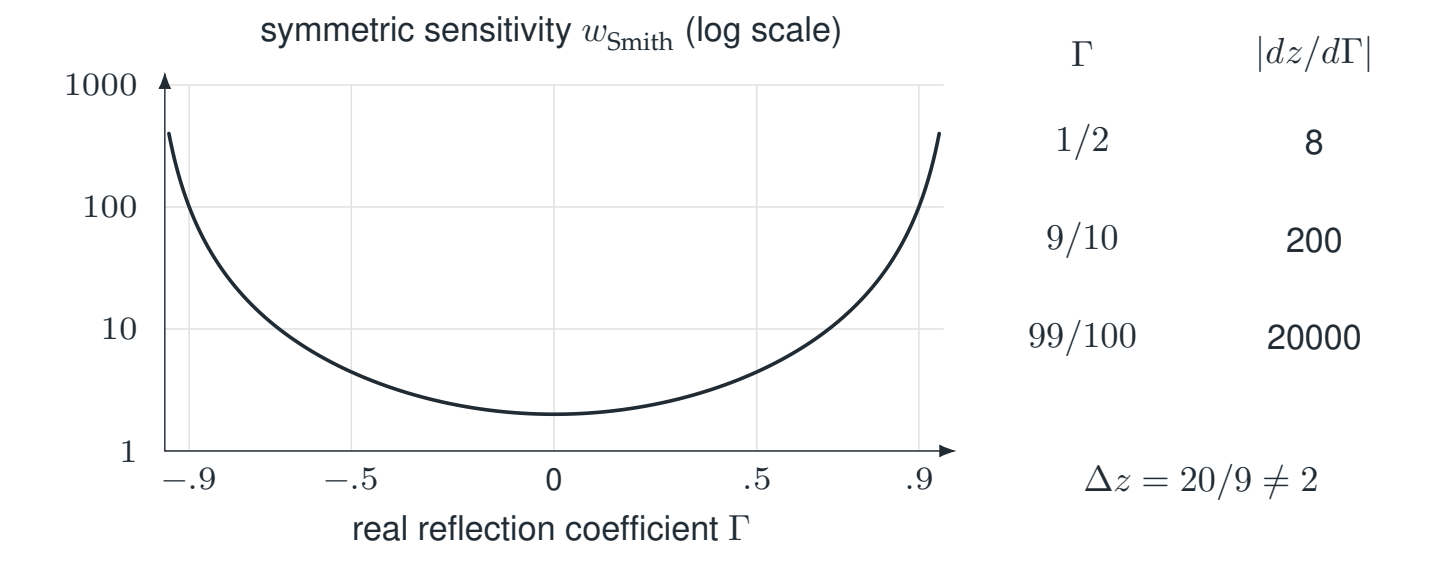
Along the real axis, three exact derivatives already show the scale change:
Reading the drawing
The curve plots the labeled sensitivity weight against reflection coefficient on a logarithmic vertical scale. A table gives exact derivative values approaching the pole.
Drawing labels and data 20 labels
Read the original labels as selectable text. Tables preserve grid relationships; other short labels are grouped compactly.
- \(-.9\)
- \(-.5\)
- 0
- \(.5\)
- \(.9\)
- \(1\)
- \(10\)
- \(100\)
- \(1000\)
symmetric sensitivity \(w_{\rm Smith}\) (log scale)
- \(1/2\)
- 8
- \(9/10\)
- 200
- \(99/100\)
- 20000
- \(\Gamma\)
- \(|dz/d\Gamma|\)
- \(\Delta z=20/9\ne2\)
- real reflection coefficient \(\Gamma\)
A differential is not the full finite-error formula
For a finite increment \(\varepsilon\), with both denominators nonzero,
At \(\Gamma=9/10\) and \(\varepsilon=1/100\), the actual increment is \(20/9\), while derivative times increment is \(2\). Both are calculated exactly. Their difference comes from using a differential in place of a finite increment. The derivative gives a first order approximation.
What a proposed weight can and cannot certify
Impedance is sensitive near \(\Gamma=1\), and admittance near \(\Gamma=-1\). The symmetric weight
reflects both chart sensitivities. Its growth motivates denser sampling near the endpoints, but does not establish an optimal grid, interpolation rule, or measurement allocation. A finite-error estimate must also control how close the perturbed point comes to either pole.
Read this as
Use the exact finite difference for an error budget. A large derivative diagnoses conditioning. Choosing an optimal algorithm requires further input.