Paper V: Smith coordinates as cyclic signal coordinates

13 Smith coordinates as cyclic signal coordinates

On this page · Visual guide: Three objects, three different questions · Permalink · Source line 1104

Let \(Z_0>0\) be a reference impedance and

\[ z=\frac{Z}{Z_0}=r+{\mathrm i} x. \]

The reflection coefficient is

\[ \boxed{ {\Gamma}=\frac{z-1}{z+1}, \qquad z=\frac{1+{\Gamma}}{1-{\Gamma}}. } \]

Classical input 13.1: Cayley geometry

The map sends the finite passive half-plane \(r\ge0\) onto the closed unit disk with \({\Gamma}=1\) omitted. Adjoining the point at infinity in impedance adds that missing boundary point; the open right half-plane maps conformally onto the open disk. Constant resistance and reactance become the familiar Smith circles. This conformal geometry is classical and is not replaced by polyphase refinement.

Permalink · Source line 1119 · Claim record · Lean coverage · Code · Worked examples

Writing \({\Gamma}=u+{\mathrm i} v\), the grid equations are

\[ \left(u-\frac{r}{1+r}\right)^2+v^2=\frac1{(1+r)^2}, \]

and, for \(x\ne0\),

\[ (u-1)^2+\left(v-\frac1x\right)^2=\frac1{x^2}. \]

Fix

\[ \omega_N=e^{2\pi{\mathrm i}/N} \]

and rotate the reflection coefficient by

\[ R_{N,k}({\Gamma})=\omega_N^k{\Gamma}. \]

Permalink · Source line 1123

Theorem 13.2: Polyphase Möbius action

Regard normalized impedance as the projective line \(\mathbb P^1({\mathbb C})={\mathbb C}\cup\{\infty\}\). For \(N\ge1\), the pullback is a globally defined projective action. In the finite chart, wherever the denominator is nonzero, it is

\[ \boxed{ T_{N,k}(z) = \frac{(1+\omega_N^k)z+(1-\omega_N^k)} {(1-\omega_N^k)z+(1+\omega_N^k)}. } \]

As maps on \(\mathbb P^1({\mathbb C})\) it satisfies

\[ T_{N,k}\circ T_{N,\ell}=T_{N,k+\ell\, (\mathrm{mod}\,N)}. \]

Read proof · Visual guide: One reflection circle, four very different impedances · Visual guide: A pole is a chart boundary, not a broken group action · Read statement and proof side by side · Permalink · Source line 1141 · Claim record · Lean coverage · Code · Worked examples

Proof of Theorem 13.2

Let \(C(z)=(z-1)/(z+1)\). Then

\[ T_{N,k}=C^{-1}\circ R_{N,k}\circ C. \]

For a division-free construction, represent a point by a nonzero pair \([u:v]\), identifying \([cu:cv]=[u:v]\) for \(c\ne0\). With \(w=\omega_N^k\), use the matrix

\[ A(w)=\frac12\begin{pmatrix}1+w&1-w\\1-w&1+w\end{pmatrix}. \]

It has determinant \(w\ne0\), preserves nonzero pairs, and commutes with rescaling, so it induces a projective map. Direct multiplication gives \(A(w)A(w')=A(ww')\) and \(A(1)=I\). Since \(\omega_N^N=1\), this proves the cyclic composition law modulo \(N\). The Cayley coordinate of \([u:v]\) is \([u-v:u+v]\), and applying \(A(w)\) changes this pair to \([w(u-v):u+v]\). This proves the conjugacy also at poles. For \([z:1]\), taking the coordinate ratio gives the displayed finite-chart formula.

Back to statement · Read statement and proof side by side · Permalink · Source line 1157 · Claim record · Lean coverage · Code · Worked examples

Corollary 13.3: Impedance–admittance is the two-phase split

For \(N=2\) and finite \(z\ne0\),

\[ \boxed{T_{2,1}(z)=z^{-1}.} \]

On the full projective line it exchanges \(0\) and \(\infty\). Thus a half-turn of the reflection disk exchanges normalized impedance and admittance.

Read proof · Visual guide: A pole is a chart boundary, not a broken group action · Read statement and proof side by side · Permalink · Source line 1169 · Claim record · Lean coverage · Code · Worked examples

Proof of Corollary 13.3

\(\omega_2=\exp(\pi{\mathrm i})=-1\), so \(A(\omega_2)[u:v]=[v:u]\). The finite ratio is \(1/z\) when \(z\ne0\); the coordinate swap also gives \([0:1]\leftrightarrow[1:0]\). No ordinary division by zero is used to represent infinity.

Back to statement · Read statement and proof side by side · Permalink · Source line 1176 · Claim record · Lean coverage · Code · Worked examples

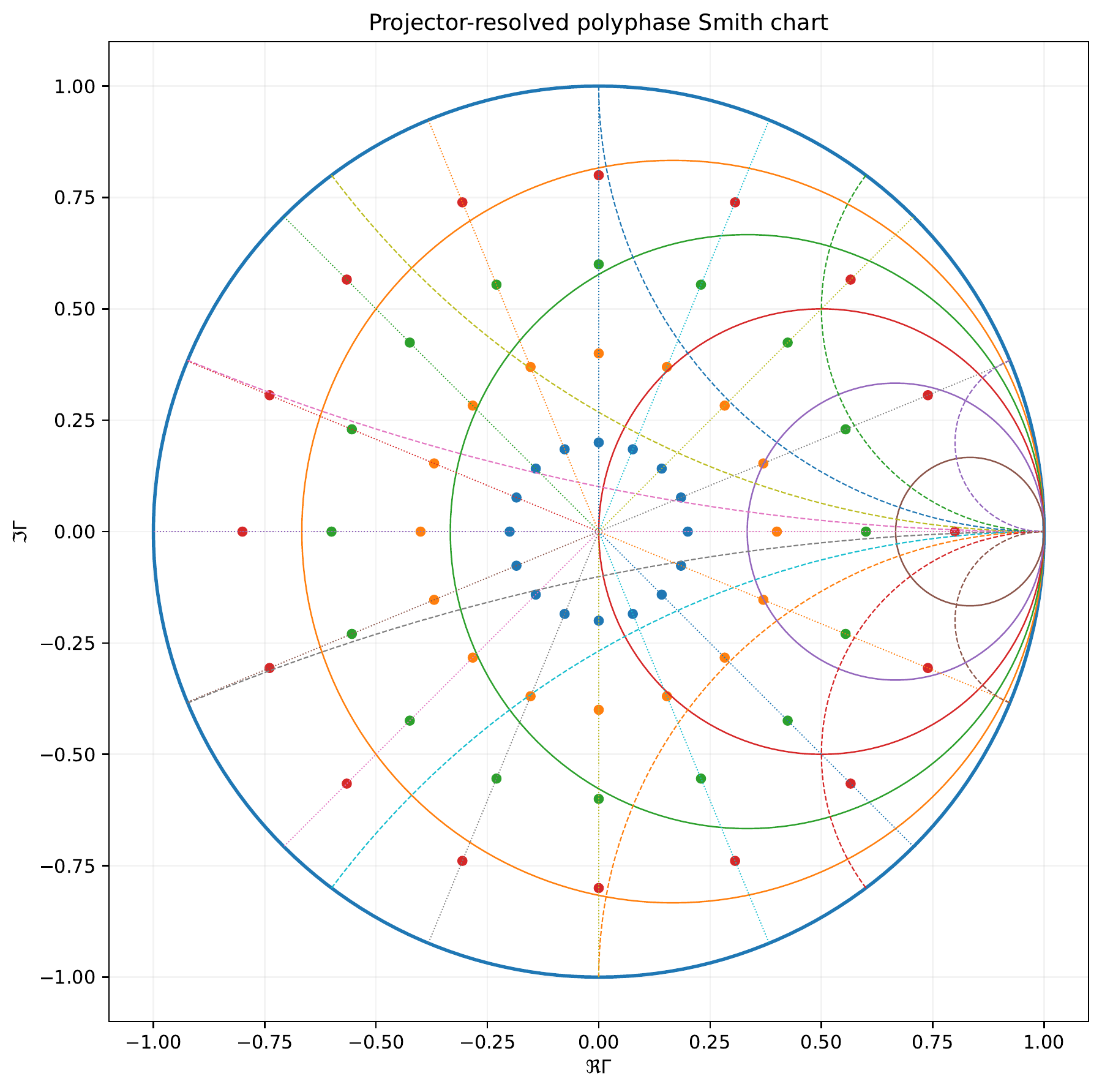
Smith reflection disk with sixteen phase rays and four radial seed orbits. — The classical Smith grid equipped with sixteen exact phase rays and four radial seed orbits. The Cayley transform creates the chart; the projector calculus supplies the nested cyclic coordinate system.

13.1 Radial seeds and physical phase

On this page · Permalink · Source line 1187

For \(0\le\rho<1\) and angle \(\theta\),

\[ {\Gamma}=\rho e^{{\mathrm i}\theta} \]

gives

\[ z(\rho,\theta) =\frac{1+\rho e^{{\mathrm i}\theta}}{1-\rho e^{{\mathrm i}\theta}}, \]

with

\[ r(\rho,\theta)=\frac{1-\rho^2}{1-2\rho\cos\theta+\rho^2}, \qquad x(\rho,\theta)=\frac{2\rho\sin\theta}{1-2\rho\cos\theta+\rho^2}. \]

A fixed \(\rho\) is a constant-mismatch circle. Refining \(N\) increases angular resolution without changing \(\rho\).

Permalink · Source line 1189

The same reflection circle at phase orders two, four, eight, sixteen and thirty-two. — The same reflection circle at phase orders \(2,4,8,16,32\). Each coarse phase ray appears in every finer grid whose order is a multiple of its order. The exact residue-projector refinement law concerns coefficient packets, not sums of impedance points.

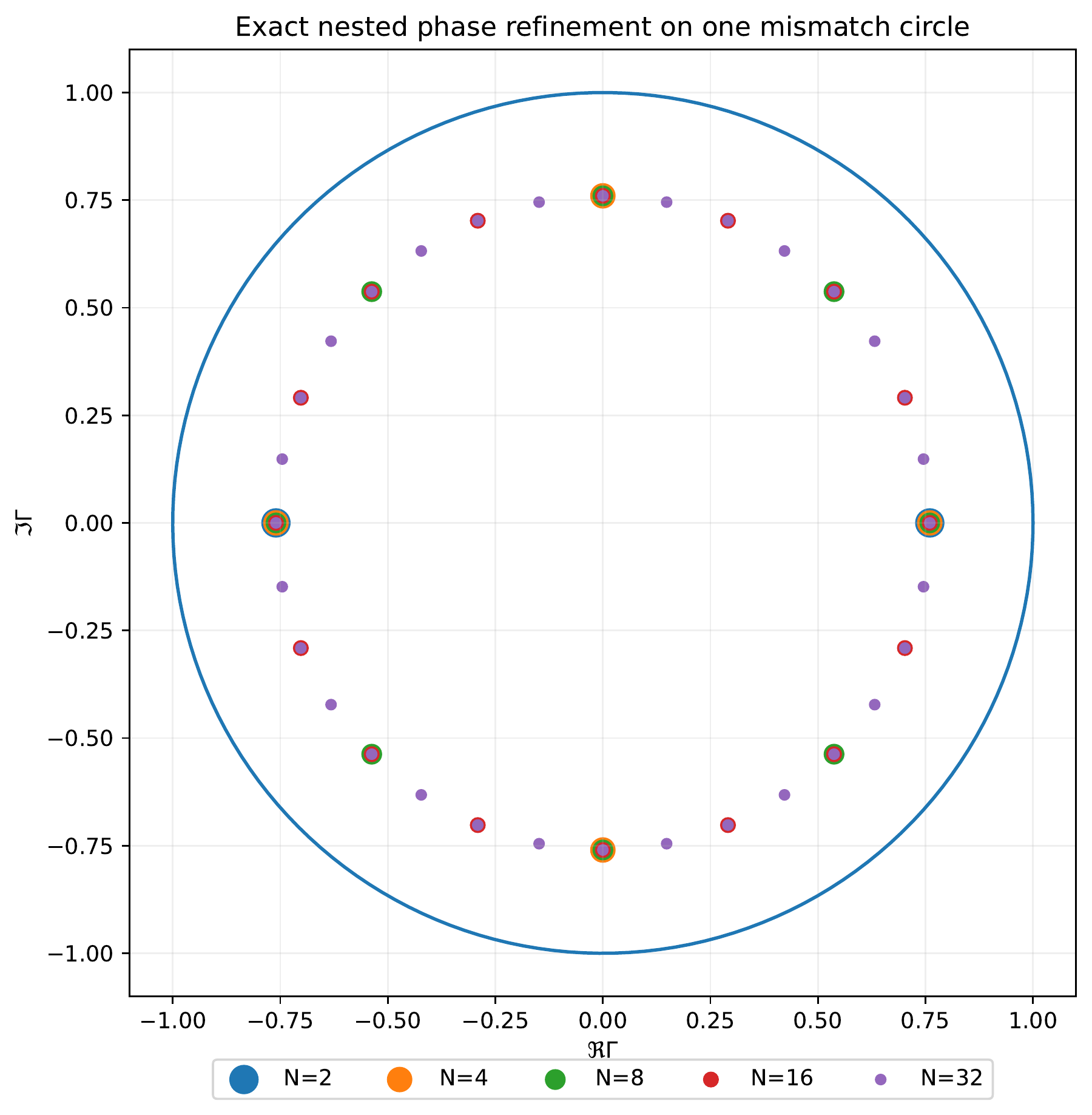
For a lossless transmission line,

\[ {\Gamma}_{\rm in}={\Gamma}_L e^{-2{\mathrm i}\beta\ell}. \]

One \(N\)-phase step corresponds to a line-length increment \(\lambda/(2N)\), up to the chosen orientation convention. Hence the phase address has a direct electrical interpretation.

Permalink · Source line 1213

Source and conversion record

Source SHA-256: 5d3c6b2e5709c37ea551eb8fd1d823e5249c5fbc411d36b806241af4df888f36

Unsupported prose commands stop the build. The mathematical expression sequence is checked against the source, with manuscript macros expanded for display.

Conversion records

Read and explore

Proofs and implementation

About this work

Other resources