
Return to the running signal \(f=s+j\). For a concrete finite calculation, use the periodic three-tap smoother
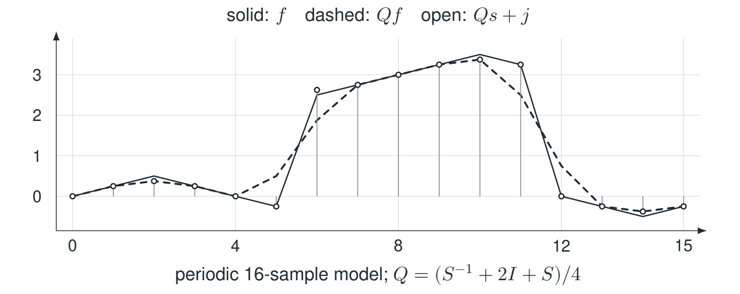
The plots compare smoothing the full signal with retaining its supplied jump packet. Every plotted sample is a rational number computed from the displayed formula.
Reading the drawing
Solid stems show the discrete target, the dashed curve shows smoothing of the full signal, and open markers show the smoothed background plus the supplied jump packet. The annotation fixes the periodic smoothing mask.
Drawing labels and data 11 labels
Read the original labels as selectable text. Tables preserve grid relationships; other short labels are grouped compactly.
- 0
- 4
- 8
- 12
- 15
- 0
- 1
- 2
- 3
- solid: \(f\) dashed: \(Qf\) open: \(Qs+j\)
- periodic 16-sample model; \(Q=(S^{-1}+2I+S)/4\)
The cancellation is the theorem
Define \(\widetilde f=Qs+j\). Then, sample by sample,
By contrast, linearity gives
The second error includes a new term caused by smoothing the discontinuity. In this finite example that term is concentrated near the two jump boundaries. The identity itself requires no linearity of the approximation applied to \(s\); linearity is used only in the comparison with \(Qf\).
The input is not discovered by subtraction
The data here include the correct \(j\). Replacing it with a wrong \(\widehat j\) retains the error \(j-\widehat j\), even when \(s\) is approximated perfectly. Multiple amplitudes and overlapping shapes are allowed if their full sum is supplied, but the identity does not estimate that sum from observations. Our finite periodic smoother is an illustration, not a new continuum approximation theorem. Its chosen boundary convention is part of the experiment.
Read this as
Known-edge reconstruction removes the jump from the approximation problem. It does not remove the need to identify the jump.