
On \([0,1]\), let \(H_\tau=\mathbf1_{[\tau,1]}\) and take
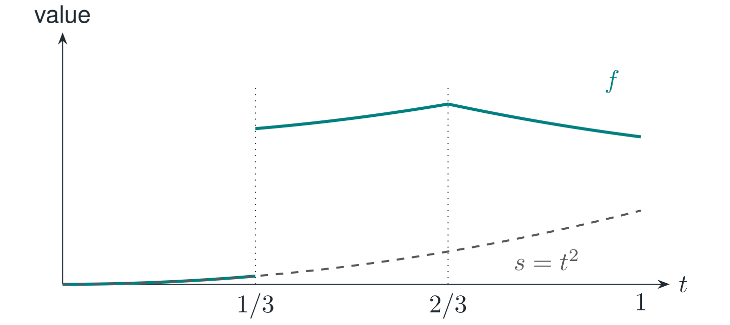
The function has a value jump \(2\) at \(1/3\) and a first-derivative jump \(-3\) at \(2/3\). Its packet and remainder are
Reading the drawing
The solid signal includes a step and a slope change above a dashed quadratic background. The horizontal axis marks the two break locations.
Drawing labels and data 7 labels
Read the original labels as selectable text. Tables preserve grid relationships; other short labels are grouped compactly.
- \(t\)
- value
- \(1/3\)
- \(2/3\)
- \(1\)
- \(f\)
- \(s=t^2\)
Evidence note from the source edition
The displayed curves are exact polynomial pieces. The solid jump is not connected across its discontinuity. The dashed curve is the global smooth remainder.
The normalization makes the trace coefficient literal
The general packet is \(\phi_{m,\tau}(t)=(t-\tau)_+^m/m!\). Its derivative of order \(m\) has a unit trace jump, while its other classical trace jumps vanish. Thus its multiplier is exactly the jump being removed, with no hidden factorial. Here the remainder has matching value and first-derivative traces and belongs to \(W^{2,p}(0,1)\) for every \(1\le p\le\infty\). Its second weak derivative is \(2\). The singular packet accounts for the distributional boundary terms that would otherwise arise at the breakpoints.
What the general theorem requires
Each piece must lie in the stated Sobolev class and possess the specified one-sided traces. Subtracting the finite trace packet then joins those pieces into a global Sobolev remainder. This is a theorem about finitely many declared breakpoints, not a representation of every possible singular measure or arbitrary image boundary.
Read this as
A value jump uses a step. A slope jump uses a ramp. The derivative order determines the packet and its normalization.