
4.9 Scaling phase diagrams for charge, particles, and local dimension
On this page · Permalink · Source line 1338
4.9.1 Exact sector size is a complexity phase variable
On this page · Permalink · Source line 1344
The statement “fixed particle number is polynomial” has a sharp extension. Let the particle number depend on the system size:
The explicit-amplitude simulation cost of one fermionic or qubit weight packet is governed by
For \(1\le k\le n\), the standard bounds
show that the growth changes continuously between polynomial and exponential regimes.
Because
write
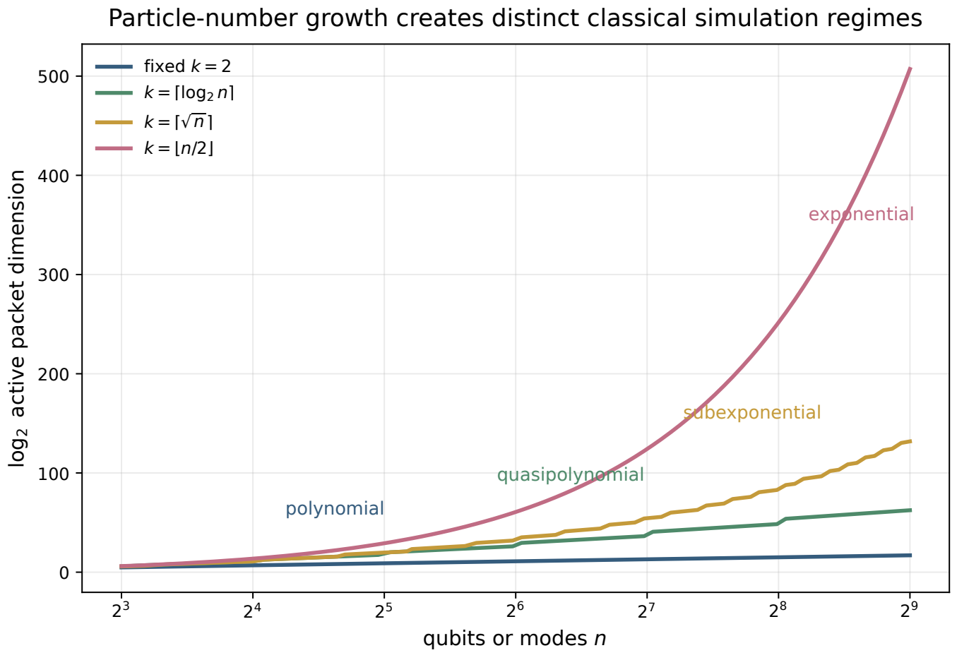
Theorem 4.11: Explicit fixed-charge phase diagram
For explicit amplitude storage in a weight-\(k(n)\) packet:
the packet dimension is polynomial in \(n\) if \(r(n)=O(1)\);
the packet dimension is superpolynomial whenever \(r(n)\to\infty\);
if \(r(n)=O(\log n)\), then
\[ D_{n,k}=2^{O((\log n)^2)}, \]so the explicit packet simulation is quasipolynomial;
if \(r(n)=O(n^\alpha)\) for a fixed \(0<\alpha<1\), then
\[ D_{n,k}=2^{O(n^\alpha\log n)}, \]which is subexponential;
if \(k(n)/n\to p\in(0,1)\), then
\[ \log_2 D_{n,k} = nH_2(k(n)/n)+O(\log n) = nH_2(p)+o(n), \]where \(H_2\) is binary entropy, and the packet remains exponential.
Proof
The upper bounds follow from Equation (4.13). If \(r=O(1)\), then \(\binom nr=O(n^r)\). Conversely, suppose \(r\to\infty\) and \(r\le n/2\). If \(r\le\sqrt n\), then
whose ratio to \(\log n\) diverges. If \(r>\sqrt n\), then
which also dominates every constant multiple of \(\log n\). For the final assertion, \(p_n=k(n)/n\) stays in a compact subinterval of \((0,1)\). Stirling's formula gives
The logarithmic term is \(O(\log n)\), uniformly on that subinterval. Continuity of \(H_2\) gives \(nH_2(p_n)=nH_2(p)+o(n)\). Replacing \(p_n\) by its limit inside an \(O(\log n)\) estimate would require a convergence rate, which is not assumed here.
Derived theorem or corollary
For the explicit occupation-amplitude representation, “few particles” means a bounded number of particles or holes. A slowly growing charge can still improve on full state-vector scaling, but it no longer guarantees membership in \(P\).
4.9.2 A bounded-excitation hierarchy
On this page · Permalink · Source line 1430
The union of the first \(K\) weight sectors has dimension
For fixed \(K\),
If \(K=O(\log n)\), the same union is quasipolynomial. This refines Corollary 3.16: bounded symmetry breaking preserves polynomial simulation, while logarithmically growing excitation gives a controlled quasipolynomial regime.
4.9.3 Bosonic and fermionic analogues
On this page · Permalink · Source line 1443
For \(N\) fermions in \(m\) modes,
For \(N\) bosons in \(m\) modes,
The same binomial analysis gives:
Corollary 4.12: Few-particle scaling
With the number of modes as the input-size parameter:
fixed \(N\) gives polynomial explicit-amplitude simulation;
\(N=O(\log m)\) gives quasipolynomial sector size;
\(N=O(m^\alpha)\), \(0<\alpha<1\), gives subexponential sector size;
finite-density fermionic sectors remain exponential.
For bosons, the statements hold in the dilute regime with the same occupation-basis access assumptions.
The adjective “polynomial” here refers to the sector dimension and efficient gate action. It does not assert that every interacting Hamiltonian has efficiently computable matrix elements or that every compact description remains closed.
4.9.4 Symmetric qudits with growing local dimension
On this page · Permalink · Source line 1468
The symmetric \(d\)-level subspace has dimension
For fixed \(d\), this is polynomial in \(n\). If \(d=d(n)\) grows, the same phase transition appears.
Proposition 4.13: Growing-local-dimension boundary
In the explicit occupation basis:
fixed \(d\) gives \(S(n,d)=O(n^{d-1})\);
\(d=O(\log n)\) gives \(S(n,d)=2^{O((\log n)^2)}\);
unbounded \(d\) is not covered by the fixed-\(d\) polynomial-collapse theorem without an additional internal compression.
Thus permutation symmetry removes the exponential tensor-product multiplicity only when the number of local levels is controlled, or when the occupation record itself admits a second compression.
4.9.5 Complexity class versus practical runtime
On this page · Permalink · Source line 1495
A polynomial sector can still have a large exponent. Fixed \(k=20\) gives \(O(n^{20})\) explicit amplitudes, which is in \(P\) but may be impractical. Conversely, a subexponential sector may be useful at moderate size without changing the formal complexity class.
A complete performance claim should therefore report both:
This is why the benchmark chapters keep wall-clock evidence separate from the dimension theorems.