
8.3 First arrival, spectral packets, algebraic rarity, and tensor regularization
On this page · Permalink · Source line 446
8.3.1 Word distance as first arrival
On this page · Permalink · Source line 455
Let \(G\) be finite and let \(S=S^{-1}\) be a symmetric generating multiset. In the right regular representation, define
Then
counts length-\(k\) words ending at \(g\).
Theorem 8.17: Endpoint Green valuation
The word distance is
Proof
Expand the resolvent as a formal power series:
The first nonzero endpoint coefficient occurs at the shortest word length.
For strictly positive integer costs, replace each generator \(s\) by the monomial \(z^{c(s)}\rho(s)\). Every coefficient then counts finitely many words of a given total cost, and the same formal inverse is defined. Zero-cost cycles require separate treatment: they can create infinitely many words of cost zero, so the ordinary counting series need not exist. The finite atlases with free gates use shortest-path search with zero-cost edges instead. Multivariate variables can track several resources when the grading gives every generator positive total degree.
8.3.2 Why eigenvalues alone are insufficient
On this page · Permalink · Source line 487
If
then
The eigenvalues and multiplicities do not determine the endpoint coefficients
Two Cayley or Schreier systems can therefore be cospectral and still have different first-arrival behavior at distinguished targets.
Principle 8.18: Embedded packet principle
For threshold questions, a spectral label is usually weaker than an embedded spectral projector. The matrix coefficients of the projector relative to the initial and target states retain positional information that multiplicities erase.
This distinction recurs in the Latin-square example discussed later. The natural commuting row, column, and symbol operators have universal eigenvalue packets at fixed order, while the embedded incidence and transition data still vary.
8.3.3 Subgroup-holonomy Fourier packets
On this page · Permalink · Source line 511
Let \(H\le G\). Let \(\mu_k(h)\) count ambient words of length \(k\) with product \(h\in H\). For every irreducible representation \(\tau\in\widehat H\), define
Fourier inversion gives
The matrix-valued Green packet
recovers every endpoint series after Fourier inversion.
The trivial representation records only the total number of loops returning to the subgroup. Nontrivial \(H\)-types retain their holonomy. This yields a hierarchy:
8.3.4 Word maps and product loci
On this page · Permalink · Source line 547
Let \(K\) be a field and let \(X\subseteq G\) be an algebraic gate family. For a fixed length \(L\), multiplication defines
The exact length-\(L\) locus is \(\mu_L(X^L)\), and the length-at-most-\(L\) locus is a finite union of such images when the gate family has finitely many components.
Theorem 8.19: Dimension per gate
Suppose every irreducible component of \(X\) has dimension at most \(r\). Then the Zariski closure of the locus reachable in at most \(L\) gates has dimension at most \(rL\).
Proof
Every component of \(X^L\) has dimension at most \(rL\). A morphism cannot increase dimension. A finite union has dimension equal to the maximum dimension of its components.
For scaled transvections, \(r=1\). This immediately yields generic lower bounds in a target variety whose dimension exceeds \(L\).
8.3.5 Generic rigidity
On this page · Permalink · Source line 565
Work over an algebraically closed field. Suppose the restricted target variety \(V\) is irreducible of dimension \(N\), every target has a restricted realization using at most \(N\) unit-cost gates, and the ambient alphabet is an algebraic family with finitely many components of dimension at most one. Then ambient realizations of length below \(N\) occupy a proper closed subset of \(V\).
Theorem 8.20: Abstract generic rigidity
Under the preceding hypotheses, there is a nonempty Zariski-open subset \(\Omega\subseteq V\) such that
The unitriangular theorem in the core chapter is a concrete instance with
8.3.6 Defect codimension
On this page · Permalink · Source line 580
If every target has restricted cost at most \(N\), then defect at least \(d\) forces ambient cost at most \(N-d\). The dimension-per-gate theorem gives
when each ambient gate carries one parameter.
Principle 8.21: Rare but amplifiable
At fixed dimension, large defects require increasingly special algebraic conditions. Under direct sums, recursive lifts, or tensor products, a point on a thin exceptional stratum can nevertheless seed a macroscopic family.
This is one of the central tensions of the subject. Catalysis is neither generic nor negligible.
8.3.7 Finite-field sparsity
On this page · Permalink · Source line 594
A word-counting analogue applies over \({\mathbb F}_q\). If the ambient alphabet has at most \(M(q-1)\) nontrivial scaled gates, then the number of targets reached in \(L\) gates is at most
When the target space has \(q^N\) points and defect \(d\) implies ambient length at most \(N-d\), the crude bound is
The estimate can be sharpened by orbit counting, stabilizers, and the geometry of word-map fibers.
8.3.8 Direct sums and monoidal amplification
On this page · Permalink · Source line 606
Suppose targets admit a direct sum \(U\oplus V\) and a homomorphism from the large restricted group onto the two factor groups sends \(U\oplus V\) to \((U,V)\). Require the aggregate generator bound
for every large restricted generator \(s\). Assume that both restricted and ambient factor circuits embed into the corresponding large model without increasing cost. Then
Indeed, projecting any word and summing the two factor bounds gives the lower bound, while concatenating the embedded factor circuits gives the upper bound. Separate one-Lipschitz projections alone do not imply this sum inequality. Under the ambient embedding assumption, the constructive upper bound is
so
One finite defect therefore gives an unbounded additive family.
8.3.9 Tensor products and normalized rates
On this page · Permalink · Source line 632
Let \(U\) have dimension \(m\) and \(V\) dimension \(n\). In linear transvection models with tree-tight certificates,
The ambient model satisfies the corresponding inequality. Normalizing by dimension gives an entropy-like law:
The normalized defect is superadditive under tensor products.
Definition 8.22: Tensor synergy
Define
Positive synergy means that the joint ambient realization improves on independent lifted circuits.
Restricted tree-tight metrics have zero tensor synergy. Ambient synergy is a possible source of collective activation.
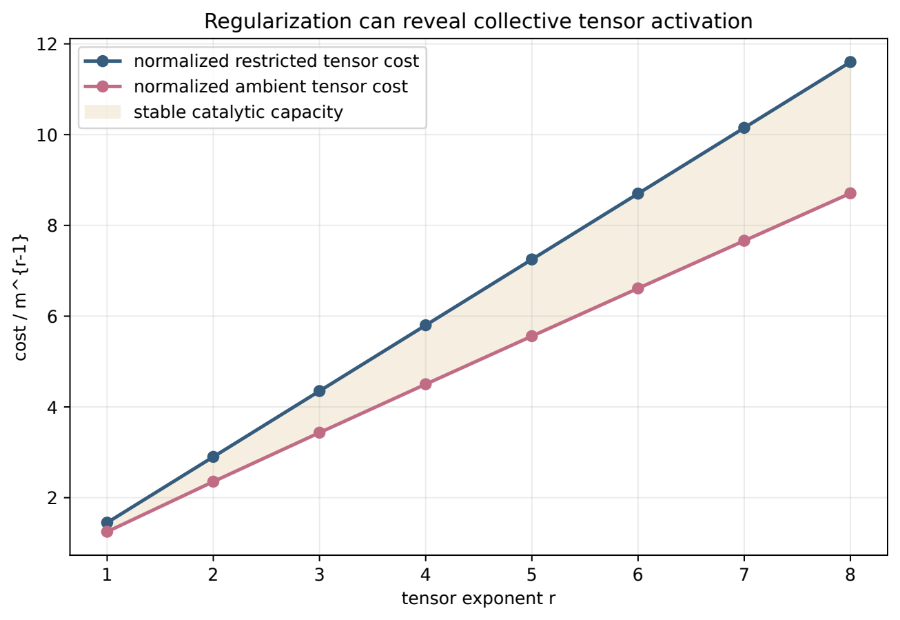
Definition 8.23: Stable tensor cost
For a size-\(m\) target \(U\), define
when the subadditivity argument applies. Define
Fekete's lemma gives the limit from the tensor subadditivity inequality.
Definition 8.24: Tensor activation
A target is tensor activated if
This is analogous to regularized capacities and asymptotic ranks. It asks whether collective synthesis can unlock a catalyst invisible in one copy.
8.3.10 Border catalysis
On this page · Permalink · Source line 692
Let \(X_{\mathrm{res}}\) and \(X_{\mathrm{amb}}\) be algebraic gate varieties. The exact product rank is
while border product rank is
The four possible comparisons are:
exact and border defects both positive,
exact defect positive but border defect zero,
one-copy defect zero but tensor-regularized defect positive,
ambient and restricted border ranks both smaller than exact ranks but by different amounts.
Each requires a separate certificate. Numerical approximation alone does not distinguish them.
8.3.11 A packet-resolved threshold principle
On this page · Permalink · Source line 714
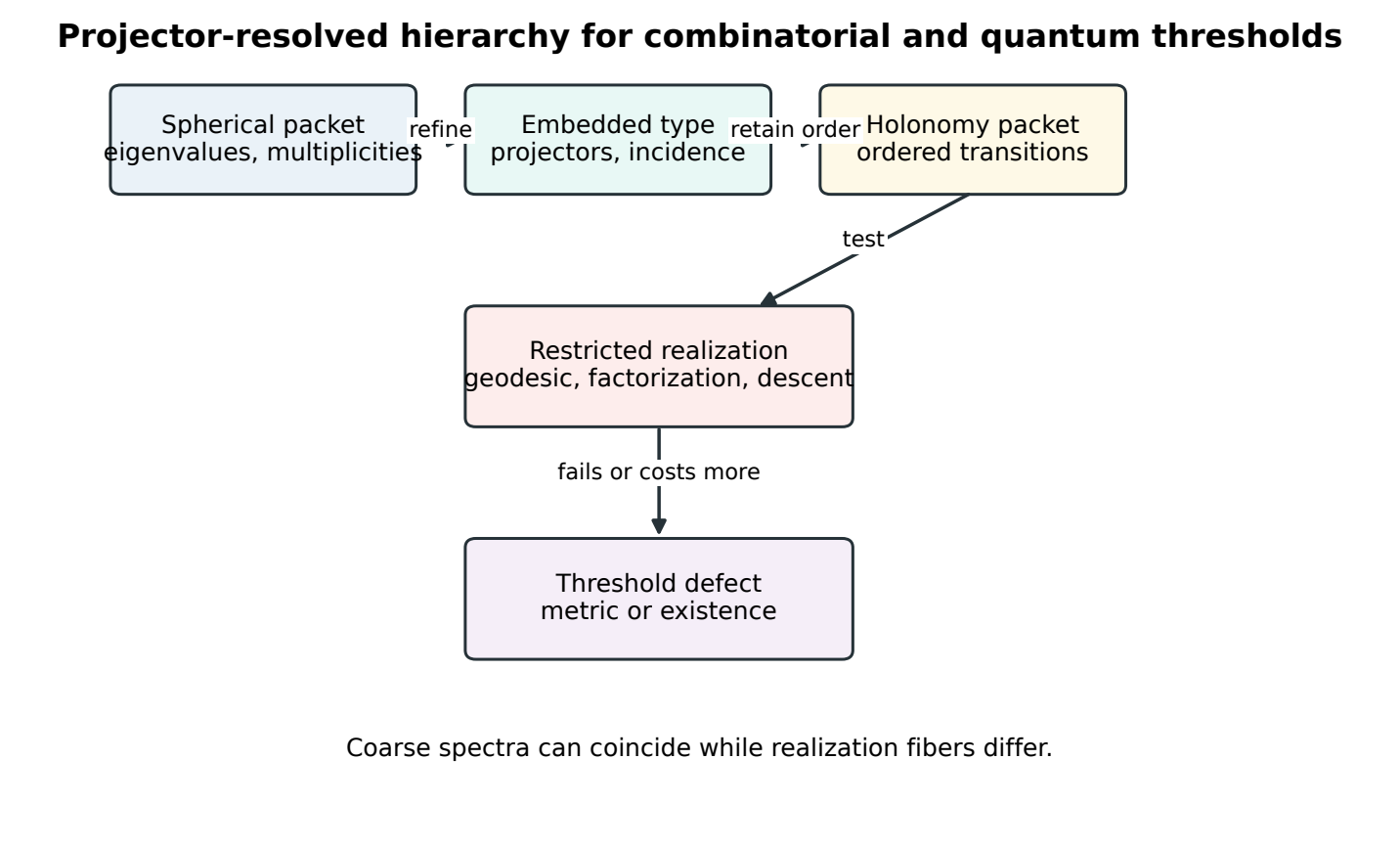
Combining the preceding constructions gives the following architecture.
A coarse commutative algebra supplies spherical spectral packets.
Embedded projectors retain incidence and endpoint position.
Noncommutative transition data record holonomy.
A realization theorem decides whether the packet has a restricted representative and at what cost.
Direct sums and tensor products propagate local defects.
Scope boundary
A packet hierarchy organizes evidence. It does not replace the final lower bound, positivity argument, orthogonality construction, or descent theorem. Classification and realization remain distinct layers.