
3.6 Moving packets, dynamic frames, and sparse transfer graphs
On this page · Permalink · Source line 412
3.6.1 Why one fixed projector is not the end of the theory
On this page · Permalink · Source line 418
The exact packet theorem in Section 3.4 follows a state inside one fixed subspace. That is sufficient for a conserved charge, but it is not necessary for classical collapse. A circuit may move through a sequence of small subspaces, or it may preserve a small packet only after a time-dependent change of coordinates. The correct object is therefore a packet schedule, not necessarily one static projector.
Definition 3.11: Packet schedule
For a circuit
on a Hilbert space \({\mathcal H}\), a packet schedule is a sequence of orthogonal projectors
It is exact when
The condition says that gate \(G_t\) maps the currently active packet into the next active packet. The dimensions may vary with time.
3.6.2 Exact dynamic-packet simulation
On this page · Permalink · Source line 440
Choose isometries
where \(D_t={\operatorname{rank}} P_t\). Define the rectangular coordinate update
Theorem 3.12: Exact dynamic-packet theorem
Suppose \(P_0{\lvert \psi_0\rangle}={\lvert \psi_0\rangle}\) and Equation (3.4) holds for every gate. Put
Then
for every \(t\).
Proof
The claim is true at \(t=0\). If the state after \(t-1\) gates is \(B_{t-1}z_{t-1}\), then
This is \(B_tz_t\).
Theorem 3.13: Polynomial moving-packet collapse
Let \(\{C_x\}\) be a polynomial-time uniform circuit family. Suppose an exact packet schedule can be produced from \(x\) in polynomial time such that:
\(\max_tD_t\le{\operatorname{poly}}(|x|)\);
the coordinate description of the initial state is computable in polynomial time;
each rectangular update \(M_t\) can be applied to polynomial precision in polynomial time;
the final acceptance probability is computable from \(z_m\) in polynomial time.
Then the language decided by the circuit family belongs to \(P\).
Proof
The simulator stores at most polynomially many coordinates at every step and applies polynomially many polynomial-time updates. Theorem 3.12 proves exactness before numerical rounding. Polynomial precision below the amplified promise gap gives a deterministic polynomial-time decision procedure.
Derived theorem or corollary
A circuit does not need one globally conserved sector. It is enough that the state follow an efficiently discoverable path through polynomial-dimensional sectors.
3.6.3 Moving frames and hidden symmetry
On this page · Permalink · Source line 501
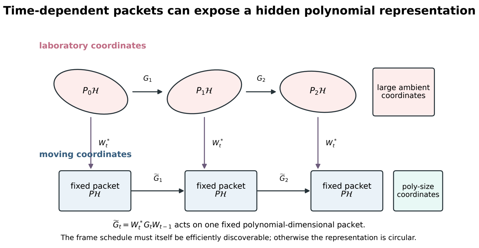
The packet schedule has a useful coordinate form. Let \(P\) be one fixed projector and let \(W_t\) be unitaries with
In the moving frame, the transformed gate is
The schedule condition is equivalent to
Corollary 3.14: Moving-frame collapse
Suppose a polynomial-time uniform circuit admits efficiently described frames \(W_t\) for which the transformed gates in Equation (3.6) preserve one fixed polynomial-dimensional packet, the initial state has efficiently computable coordinates in \(W_0P{\mathcal H}\), and their restricted matrices and the transformed final measurement are efficiently computable. Then the circuit family is classically simulable in polynomial time.
This is the appropriate theorem for a symmetry that changes orientation with time. Examples to test include Clifford frames, Gaussian mode frames, rotating spin axes, and gauge-fixed local coordinates.
Scope boundary
The frame must be independently discoverable and efficiently usable. Choosing \(W_t=G_t\cdots G_1\) makes the transformed state trivial but is circular: computing that frame is the original simulation problem. The theorem is useful only when the frames have a compact classical description and their restricted actions can be computed without constructing the full state.
3.6.4 Sparse packet-transfer graphs
On this page · Permalink · Source line 534
Let
be an orthogonal packet decomposition. Write the gate blocks as
Starting from an active packet set \(S_0\), define recursively
Corollary 3.15: Reachable packet-graph collapse
Suppose the packet sets \(S_t\) and nonzero transfer blocks are computable in polynomial time, and
for every \(t\). If all active block updates and the final measurement are efficiently computable, then the circuit family is classically polynomial-time simulable.
Proof
Take
The definition of \(S_t\) gives \(G_tP_{t-1}=P_tG_tP_{t-1}\). Apply Theorem 3.13.
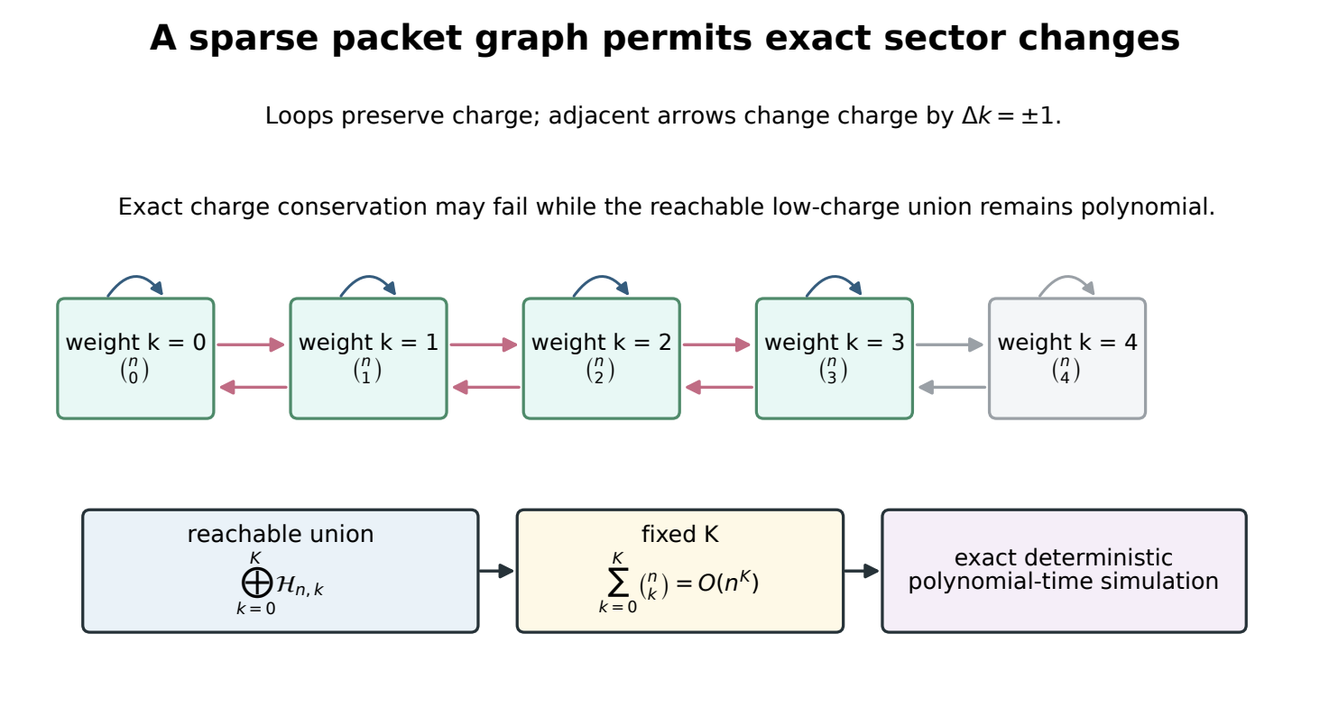
This theorem permits exact sector changes. What matters is not that one charge be fixed, but that the union of reachable sectors remain polynomial.
Corollary 3.16: Bounded-excitation collapse
Consider \(n\) qubits and suppose the initial state and every circuit prefix are certified to lie in
for a fixed constant \(K\). If initialization, the gate actions, and the measurement are computable in polynomial time in the occupation basis, then the circuit family lies in \(P\), even when individual gates change excitation number.
Proof
The active dimension is
Let \(P\) project onto \({\mathcal H}_{\le K}\). By the hypothesis on the actual circuit prefixes, \(P\psi_t=\psi_t\) at every step. Consequently \(PG_tP\psi_{t-1}=G_t\psi_{t-1}\) on the evolving state, even if the gate does not preserve all of \(P{\mathcal H}\). The restricted update therefore reproduces that trajectory exactly. The hypothesis supplies efficient initialization, updates, and measurement in these polynomially many coordinates.
For example, a fixed-weight input followed by only a constant number of pair-creation or pair-annihilation events remains in a constant collection of low-weight sectors. Exact number conservation is therefore stronger than necessary.
3.6.5 Approximate dynamic packets
On this page · Permalink · Source line 604
Define the one-step leakage from the scheduled packet by
Let
Theorem 3.17: Dynamic sum-of-leakages bound
For an initial unit vector in \(P_0{\mathcal H}\),
For any acceptance operator \(0\le M\le I\), the corresponding acceptance probabilities differ by at most
Proof
A telescoping expansion inserts \(G_t-\widehat G_t\) at one time. On \(P_{t-1}{\mathcal H}\) this difference equals \((I-P_t)G_tP_{t-1}\), while all other unitary or projected factors have norm at most one. Summing the operator norms proves the state bound. If \(\psi\) and \(\phi\) have norm at most one, then
Corollary 3.18: Approximate moving-packet collapse
If the scheduled dimensions and updates are polynomial and
then, after ordinary promise-gap amplification, the circuit family remains deterministically classically simulable in polynomial time.
The result is conservative but fully composable. It extends the fixed-projector estimate of Section 3.5 to moving frames and changing packet sets.
3.6.6 An adaptive certificate from discarded state vectors
On this page · Permalink · Source line 655
The operator-norm leakage certificate is uniform over every input in a packet. An adaptive simulator can use a less expensive certificate that follows its actual approximate state. The discarded vector must be accounted for before any normalization.
Theorem 3.19: Adaptive discarded-state certificate
Let \(G_1,\ldots,G_m\) be unitary operators on a finite-dimensional Hilbert space, and let \(\psi_0=\phi_0\) be a unit vector. At each step choose an orthogonal projector \(P_t\), possibly as a function of the previously computed approximate states. Define
Then
For an effect \(0\le M\le I\),
No renormalization of \(\phi_t\) is performed. The second quadratic form is an unnormalized acceptance estimate.
Proof
Fix the projectors chosen during the particular run. Put \(d_t=(I-P_t)G_t\phi_{t-1}\). Subtraction gives the exact recurrence
Since \(\psi_0-\phi_0=0\), iteration yields
Every unitary product preserves norm, so the triangle inequality proves the state estimate. Also \(\|\psi_m\|=1\) and \(\|\phi_m\|\le1\) because each projector is contractive. Expanding the difference of the two quadratic forms and using \(\|M\|\le1\) gives the factor two. This proof applies to the chosen run even when the projectors were selected adaptively.
Example 3.20: A rational two-step certificate
Take
Using \(G_1=G_2=G\) and \(P_1=P_2=P\) gives
The squared state error is \(832/625\), below \((\eta_1+\eta_2)^2=1024/625\). The rational validation script checks these values exactly. The deliberately large tail illustrates a valid but loose certificate, not an efficient approximation.
The theorem closes global error accounting for any adaptive projection run whose discarded vectors or certified norm bounds can be computed. It does not prove that the retained representation stays polynomial, that the discarded norm is cheap to evaluate, or that a small tail can always be found. Those are separate algorithmic obligations. This is a written theorem with exact finite controls, not an additional Lean formalization.