
On \({\mathbb C}^3={\mathbb C}{\left|0\right\rangle}\oplus{\mathbb C}^2\), use \(C_a=0\oplus\sigma_a\) for \(a=x,y,z\). The common kernel is \({\mathbb C}{\left|0\right\rangle}\), and the full algebra closes:
These are uncompressed identities. They supply an actual closure test in the quotient by the constraint span, unlike the automatic compressed zero on the physical kernel.
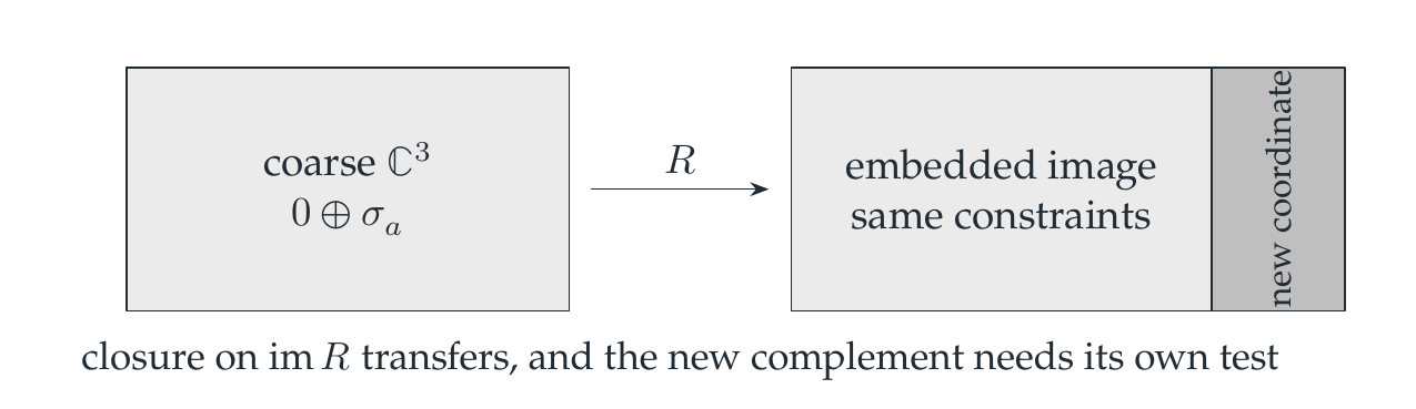
Reading the drawing
The arrow maps the coarse box into the shaded image inside the larger box. A separately marked new coordinate lies outside that image. The note distinguishes transferred closure on the image from the test still needed on the complement.
Drawing labels and data 5 labels
Read the original labels as selectable text. Tables preserve grid relationships; other short labels are grouped compactly.
coarse \({\mathbb C}^3\)
\(0\oplus\sigma_a\)
- \(R\)
embedded image
same constraints
- new coordinate
closure on \(\operatorname{im}R\) transfers, and the new complement needs its own test
Exact transport holds on the coarse image
Embed by the coordinate isometry \(R:{\mathbb C}^3\to{\mathbb C}^4\) and set \(\widetilde C_a=C_a\oplus1\). Then \(\widetilde C_aR=RC_a\), so
The coarse physical vector maps into the fine common kernel. However, the same prescribed Pauli structure does not close on the whole fine level: on the added coordinate the commutator is zero, whereas \(2{\mathrm i}\widetilde C_z\) is \(2{\mathrm i}\). Exact transport constrains the image of \(R\) and leaves its orthogonal complement as separate data.
An approximate residual is also explicit
Perturb only \(\widetilde C_x\) by \((1/10){\left|0\right\rangle}{\left\langle0\right|}\). For the unit coarse physical vector, the fine constraint residual is exactly \(1/10\). The intertwining defect has the same norm. The general result for approximate transport controls these residuals and commutator errors using the defect sizes and a common bound on the constraint norms. A nonzero anomaly remains an error that must be controlled.
The retained checks verify all three coarse commutators, the isometry, each constraint intertwining, all nine commutator transports, and the residual. The added coordinate provides a counterexample to extending the identity on the image to the whole space. Unbounded constraints would additionally require a common invariant domain.
Read this as
Closure is a statement about the operator algebra. Refinement intertwining transports it to the embedded image. The new degrees of freedom require their own control.