
II.1 Introduction
On this page · Visual guide: Three objects, three questions · Permalink · Source line 1
Quantum mechanics repeatedly uses the same operation. A Hilbert space is split into sectors, an operator is resolved between those sectors, and the pieces are propagated or recombined. Symmetry sectors, eigenspaces, syndrome spaces, adiabatic subspaces, and retained model spaces are familiar examples. This article treats them as instances of one finite packet calculus.
The elementary coordinate object is a complete family of orthogonal projectors
Every vector has packet coordinates \(P_a\psi\). Every operator has transfer blocks
These identities are simple. Their value appears when the same coordinates are used across representation theory, circuits, channels, error correction, effective dynamics, and geometric limits.
Quantum information and operator theory in finite dimensions provide the standard background [NielsenChuang2010], [Watrous2018], [Bhatia1997]. Finite group projectors come from character theory [Serre1977], [FultonHarris1991]. Moving spectral subspaces and geometric phase originate in the work of Kato, Berry, Wilczek, and Zee [Kato1950], [Kato1995], [Berry1984], [WilczekZee1984]. Completely positive maps and quantum dynamical semigroups are treated in [Stinespring1955], [Choi1975], [Kraus1983], [Lindblad1976]. Exact error correction is governed by the Knill Laflamme condition [KnillLaflamme1997], [SchumacherNielsen1996], [BenyKempfKribs2007]. Projection methods and hidden state memory are linked by the Feshbach, Nakajima, and Zwanzig constructions [Feshbach1958], [Nakajima1958], [Zwanzig1960], [BravyiDiVincenzoLoss2011].
The first part begins with quantum seeds. A state is cyclic only relative to a declared observable algebra. For an algebra in multiplicity form, the local orbit dimension is controlled by the rank of a coefficient matrix. This recovers the relation between Schmidt rank and the dimension reached by local operations. The finite group section then constructs central isotypic projectors. Cyclic symmetry gives a sharper charge selection rule. An operator with charge \(q\) can move a state only from packet \(j\) to packet \(j+q\).
A circuit is resolved by inserting the identity between successive gates. This produces a sum over packet paths. The target probability contains diagonal path terms and interference between distinct paths. Symmetry can remove entire path families before any matrix multiplication is performed. Unitarity gives exact row and column relations among the transfer blocks.
The moving packet section treats time dependent projectors. The canonical generator
is skew adjoint and transports every packet. In the moving frame, the physical Hamiltonian acquires the geometric term \(-{\mathrm i} W(t)^*\dot W(t)\). The leakage estimate must account for the motion of the packet itself. The physical coupling \(QHP\) is therefore replaced by
This is the exact finite distinction between following a moving subspace and remaining in a fixed one.
Density matrices require separate packet labels for their output and input coordinates. The superoperators
form a complete orthogonal packet system on Hilbert Schmidt operator space. Dephasing is the diagonal projection. Every channel has input and output superblocks, with the same composition law as ordinary matrix blocks. A covariant channel preserves the isotypic packets of the conjugation action. In the cyclic case these are coherence orders. The Choi matrix carries the equivalent symmetry under \(U\otimes\overline U\).
Error correction is expressed through compression to a code. Let \(P\) be the code projector. The class of \(PAP\) modulo scalar multiples of \(P\) measures the obstruction to making \(A\) undetectable within the code. The Knill Laflamme criterion says that this obstruction vanishes for every product \(E_a^*E_b\) from the error family. Diagonalizing the resulting positive coefficient matrix produces orthogonal syndrome packets and an explicit recovery on the error span.
The effective dynamics section returns to ordinary Hilbert space packets. Schur complementation gives the exact retained resolvent and a frequency dependent self energy. The same hidden block gives a causal memory kernel in time. For a self adjoint hidden Hamiltonian, the self energy has a fixed sign in the upper half plane, and the time kernel is positive definite. Uniform spectral separation gives direct bounds that can be carried through a refinement tower.
The geometric part develops two finite constructions. A strictly positive contraction gives a reflection positive Hankel kernel, and its logarithm reconstructs a nonnegative Hamiltonian. A finite Laplacian gives a heat trace from which the spectral dimension is defined at each diffusion scale. The article proves convergence from periodic lattices to the continuum torus at every fixed positive diffusion time. Poisson summation then determines the continuum dimension as diffusion time tends to zero.
Constraint closure needs a different obstruction. If \(C_a\) are self adjoint constraints and \(P_{{\mathrm{phys}}}\) projects onto their common kernel, then
holds automatically. This compression cannot test closure. The correct finite obstruction is the class of \([C_a,C_b]\) in the quotient of \({\operatorname{End}}({\mathcal H})\) by the span of the constraints. Vanishing means that the constraint span is closed under commutators.
The last part gives two theorems for towers of bounded Hamiltonians. Exactly compatible finite Hamiltonians with a uniform norm bound define a bounded self adjoint operator on the Hilbert direct limit. When successive bounded self adjoint Hamiltonians on a common Hilbert space have norm summable differences, they converge to a bounded self adjoint limit. Their unitary evolutions, and their Euclidean evolutions under the stated positivity assumption, converge uniformly on bounded time intervals. Reflection positivity and closure with fixed structure coefficients pass to the limit under the stated convergence assumptions.
These results do not construct an interacting continuum quantum field theory. They do not prove anomaly freedom on an unbounded common domain, Osterwalder Schrader reconstruction for a continuum measure, an Einstein infrared action, or a positive massless spin two sector. Each of those conclusions needs hypotheses absent from the finite calculations.
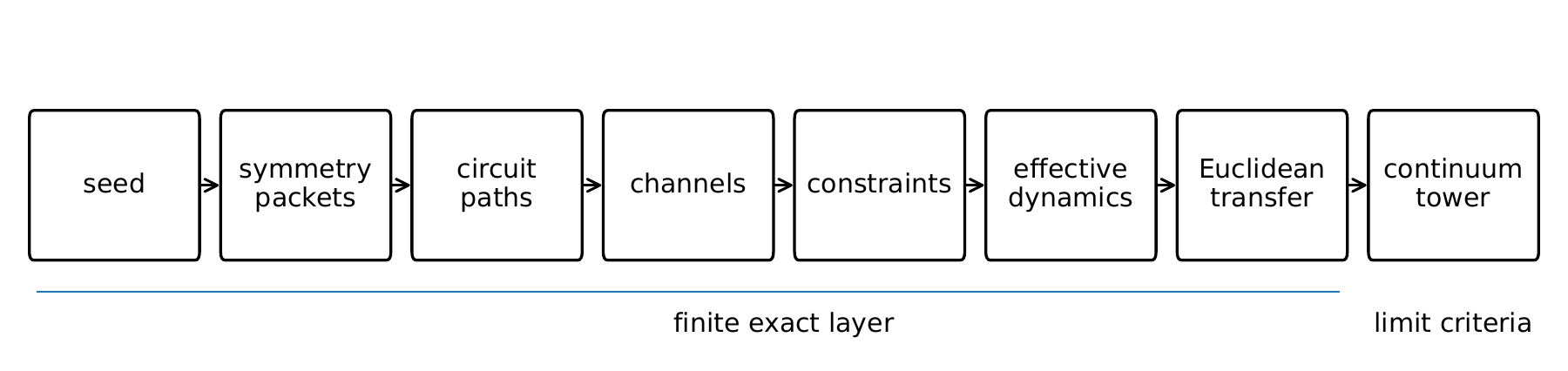
Text description
Boxes progress through seed, symmetry packets, circuit paths, channels, constraints, effective dynamics, Euclidean transfer, and continuum tower. A line groups the finite exact layer separately from the limit criteria at the final stage.
| Object | Packet coordinate | Exact structural condition |
|---|---|---|
| State | \(P_a\psi\) | completeness of the projector family |
| Operator | \(P_bAP_a\) | block multiplication |
| Circuit | intermediate packet path | insertion of complete resolutions |
| Density matrix | \(P_a\rho P_b\) | two sided operator packets |
| Channel | superoperator block | complete positivity and covariance when declared |
| Code | syndrome packet | scalar compression of error products |
| Effective model | Feshbach map | invertibility of the hidden resolvent |
| Euclidean model | positive transfer matrix | positivity and self adjointness |
| Constraint system | quotient obstruction | commutator closure modulo the constraint span |
| Continuum tower | direct or norm limit | compatibility plus explicit convergence |
II.2 Quantum seeds and observable algebras
On this page · Permalink · Source line 85
Definition II.2.1: Finite quantum seed system
A finite quantum seed system is a triple
where \({\mathcal H}\) is a finite dimensional Hilbert space, \({\mathcal A}\subseteq{\operatorname{End}}({\mathcal H})\) is a unital star subalgebra, and \(S\subseteq{\mathcal H}\) is a finite set. Its generated hull is
The seed set is cyclic when \({\mathcal A} S={\mathcal H}\). The quantum seed rank is the least cardinality of a cyclic seed set.
Visual guide: The objects on the page · Permalink · Source line 87 · Claim record · Lean coverage · Code · Worked examples
The algebra is part of the data. A vector may be cyclic for \({\operatorname{End}}({\mathcal H})\) and fail to be cyclic for a restricted observable or gate algebra.
Let
act on
Assume \(d_r,m_r\ge1\) for each displayed block. For an empty block family, the seed rank and the displayed finite supremum are defined as zero. A vector in one block is identified with a \(d_r\) by \(m_r\) coefficient matrix.
Theorem II.2.2: Orbit dimension of one seed
For integers \(d\ge1\), \(m\ge0\), and the action of \(M_d({\mathbb C})\otimes I_m\) on \({\mathbb C}^d\otimes{\mathbb C}^m\), let \(C_\psi\) be the coefficient matrix of \(\psi\). Then
The vector is cyclic exactly when \({\operatorname{rank}} C_\psi=m\).
Read proof · Visual guide: Entanglement changes the local span · Read statement and proof side by side · Permalink · Source line 119 · Claim record · Lean coverage · Code · Worked examples
Proof of Theorem II.2.2
Under the coefficient matrix identification, \((A\otimes I_m)\psi\) corresponds to \(AC_\psi\). Every row of \(AC_\psi\) lies in the row space of \(C_\psi\). Conversely, a matrix whose rows lie in that row space equals \(AC_\psi\) for a suitable \(A\). There are \(d\) independent row choices in a space of dimension \({\operatorname{rank}} C_\psi\). The orbit dimension is therefore \(d{\operatorname{rank}} C_\psi\). It equals \(dm\) exactly when \(C_\psi\) has full column rank.
Back to statement · Read statement and proof side by side · Permalink · Source line 129 · Claim record · Lean coverage · Code · Worked examples
Theorem II.2.3: Quantum seed rank
For the displayed multiplicity decomposition,
Read proof · Visual guide: Why one seed is not always enough · Read statement and proof side by side · Permalink · Source line 133 · Claim record · Lean coverage · Code · Worked examples
Proof of Theorem II.2.3
A single seed contributes a row space of dimension at most \(d_r\) to the \(r\)th multiplicity factor. Hence \(k\) seeds cover at most \(kd_r\) multiplicity directions, which gives the lower bound.
Set
For each \(r\), partition a basis of \({\mathbb C}^{m_r}\) into at most \(k\) groups of size at most \(d_r\). Choose the coefficient matrix of the \(j\)th seed so that its row space spans the \(j\)th group. The combined row spaces span every multiplicity factor. The preceding theorem then shows that the \(k\) seeds generate every summand.
Back to statement · Read statement and proof side by side · Permalink · Source line 143 · Claim record · Lean coverage · Code · Worked examples
Corollary II.2.4: Local orbit and Schmidt rank
Let \(\psi\in{\mathcal H}_A\otimes{\mathcal H}_B\), let \(d_A=\dim{\mathcal H}_A\ge1\), and let \(r\) be the Schmidt rank of \(\psi\). Then
Local operators on \(A\) generate the whole bipartite Hilbert space exactly when the reduced state on \(B\) has full support.
Read proof · Visual guide: Entanglement changes the local span · Read statement and proof side by side · Permalink · Source line 153 · Claim record · Lean coverage · Code · Worked examples
Proof of Corollary II.2.4
The Schmidt rank is the rank of the coefficient matrix in any product basis. Substituting that rank into Theorem II.2.2 gives the stated orbit dimension.
Back to statement · Read statement and proof side by side · Permalink · Source line 163 · Claim record · Lean coverage · Code · Worked examples
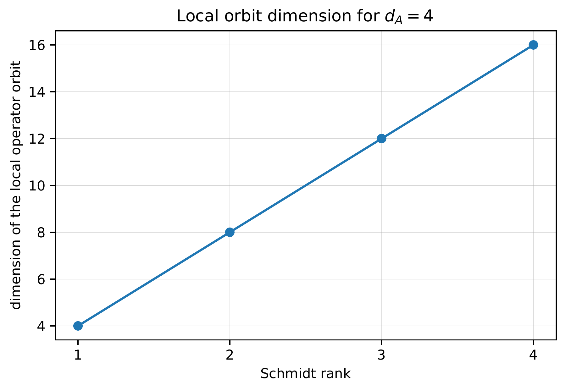
Text description
With the displayed local dimension fixed at four, the plotted orbit dimensions are four, eight, twelve, and sixteen at Schmidt ranks one through four. The connected points illustrate the finite rank formula under the chapter assumptions.
Proposition II.2.5: Computational address orbit
For \(n\) qubits, let
and let \(X_j\) be the Pauli \(X\) operator on the \(j\)th qubit. Then
is the computational basis.
Read proof · Visual guide: One seed, eight addresses · Read statement and proof side by side · Permalink · Source line 174 · Claim record · Lean coverage · Code · Worked examples
Proof of Proposition II.2.5
The addressed vector is \({\left|a_1\cdots a_n\right\rangle}\). Distinct binary addresses produce the \(2^n\) distinct basis vectors.
Back to statement · Read statement and proof side by side · Permalink · Source line 189 · Claim record · Lean coverage · Code · Worked examples
Remark II.2.6
The seed rank records generation by a declared algebra. It does not measure circuit depth, locality cost, control complexity, or physical reachability under a restricted time dependent Hamiltonian.
II.3 Symmetry packets and selection rules
On this page · Permalink · Source line 197
Let \(G\) be a finite group and let
be a unitary representation. Write \(\widehat G\) for the set of irreducible unitary representations. For \(\lambda\in\widehat G\), let \(d_\lambda\) and \(\chi_\lambda\) denote its dimension and character.
Theorem II.3.1: Finite group isotypic projectors
The operators
are orthogonal projectors. They satisfy
The range of \(P_\lambda\) is the \(\lambda\) isotypic component of \({\mathcal H}\).
Read proof · Visual guide: Nonabelian packets carry multiplicity · Read statement and proof side by side · Permalink · Source line 205 · Claim record · Lean coverage · Code · Worked examples
Proof of Theorem II.3.1
Complete reducibility gives a unitary decomposition
On the \(\mu\) summand, the displayed average is central in the irreducible representation \(\pi_\mu\), so it is a scalar by Schur's lemma. Taking its trace and applying character orthogonality shows that the scalar is one when \(\mu=\lambda\) and zero otherwise. The asserted identities follow on the direct sum.
Back to statement · Read statement and proof side by side · Permalink · Source line 223 · Claim record · Lean coverage · Code · Worked examples
The central projectors separate irreducible types but do not choose coordinates inside the representation factor. Matrix units provide that finer resolution.
Theorem II.3.2: Representation matrix units
Fix an irreducible unitary representation \(\pi_\lambda:G\to U(d_\lambda)\) and an orthonormal basis of its representation space. Define
Then
and
Read proof · Visual guide: Nonabelian packets carry multiplicity · Read statement and proof side by side · Permalink · Source line 241 · Claim record · Lean coverage · Code · Worked examples
Proof of Theorem II.3.2
Apply the matrix coefficient form of Schur orthogonality to the two group averages. It gives the matrix unit multiplication law. Unitarity gives the adjoint relation after replacing \(g\) by \(g^{-1}\). Summing the diagonal coefficients gives the character average in Theorem II.3.1.
Back to statement · Read statement and proof side by side · Permalink · Source line 264 · Claim record · Lean coverage · Code · Worked examples
II.3.1 Cyclic charge packets
On this page · Permalink · Source line 268
Let \(N\ge1\) be an integer, \(S\) unitary with \(S^N=I\), and \(\omega={\mathrm e}^{2\pi{\mathrm i}/N}\).
Corollary II.3.3: Cyclic charge projectors
The operators
form a complete orthogonal packet system and satisfy
Read proof · Visual guide: Four phases resolve a cyclic shift · Visual guide: One calculation of transfer to the opposite site · Read statement and proof side by side · Permalink · Source line 272 · Claim record · Lean coverage · Code · Worked examples
Proof of Corollary II.3.3
Apply Theorem II.3.1 to the cyclic group. Its irreducible representations are the one dimensional characters \(r\mapsto\omega^{jr}\).
Back to statement · Read statement and proof side by side · Permalink · Source line 289 · Claim record · Lean coverage · Code · Worked examples
Definition II.3.4: Operator charge
An operator \(A\in{\operatorname{End}}({\mathcal H})\) has cyclic charge \(q\in{\mathbb Z}/N{\mathbb Z}\) when
Permalink · Source line 293 · Claim record · Lean coverage · Code · Worked examples
Theorem II.3.5: Charge selection rule
If \(A\) has charge \(q\), then
unless \(k=j+q\) in \({\mathbb Z}/N{\mathbb Z}\). In fact,
Read proof · Read statement and proof side by side · Permalink · Source line 300 · Claim record · Lean coverage · Code · Worked examples
Proof of Theorem II.3.5
For \(x\in P_j{\mathcal H}\),
Thus \(Ax\in P_{j+q}{\mathcal H}\). The block statement follows.
Back to statement · Read statement and proof side by side · Permalink · Source line 311 · Claim record · Lean coverage · Code · Worked examples
Corollary II.3.6: Charge addition
If \(A\) and \(B\) have charges \(q\) and \(r\), then \(AB\) has charge \(q+r\). The adjoint \(A^*\) has charge \(-q\).
Read proof · Read statement and proof side by side · Permalink · Source line 321 · Claim record · Lean coverage · Code · Worked examples
Proof of Corollary II.3.6
Conjugation by \(S\) is a star automorphism. Applying it to \(AB\) adds the two charges, while applying it to \(A^*\) changes the sign of the charge.
Back to statement · Read statement and proof side by side · Permalink · Source line 325 · Claim record · Lean coverage · Code · Worked examples
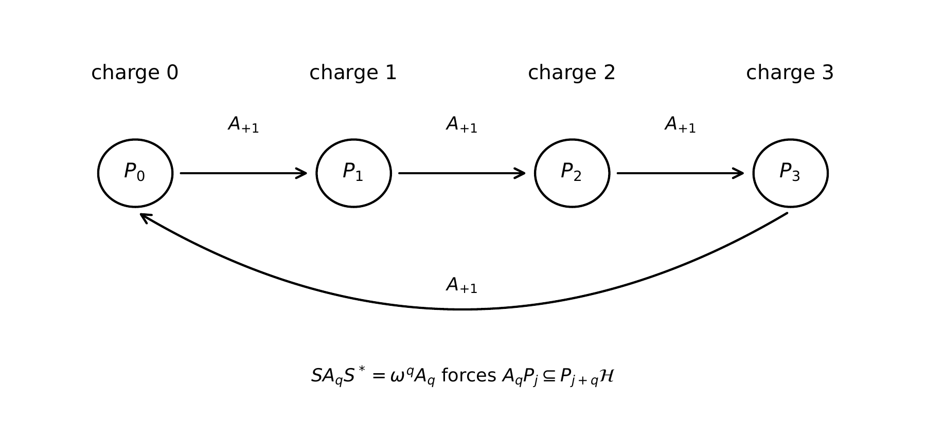
Text description
Four packet nodes P0 through P3 are arranged in a cycle. Arrows labeled with the charge-one operator go to the next packet and return from P3 to P0. The accompanying identity restricts transfer to those allowed blocks.
II.3.2 Tensor refinement
On this page · Permalink · Source line 336
Suppose the \(a\)th tensor factor carries a cyclic packet family
The fine tensor packets are
Theorem II.3.7: Tensor charge refinement
For \(r\in{\mathbb Z}/N{\mathbb Z}\), define
Then the \(P_r^{\rm total}\) form a complete orthogonal packet system. Every total charge packet is the exact sum of its fine tensor descendants.
Read proof · Visual guide: A coarse packet can still contain coherence · Read statement and proof side by side · Permalink · Source line 349 · Claim record · Lean coverage · Code · Worked examples
Proof of Theorem II.3.7
The fine tensor projectors are mutually orthogonal and sum to the identity. The total residue classes partition the fine address set. Summing the fine projectors over each class gives the result.
Back to statement · Read statement and proof side by side · Permalink · Source line 360 · Claim record · Lean coverage · Code · Worked examples
Corollary II.3.8: Tensor selection rule
If \(A_a\) has local charge \(q_a\), then
has total charge \(q_1+\cdots+q_m\).
Read proof · Visual guide: A coarse packet can still contain coherence · Read statement and proof side by side · Permalink · Source line 364 · Claim record · Lean coverage · Code · Worked examples
Proof of Corollary II.3.8
Conjugate the tensor product by the total cyclic symmetry and multiply the local phase factors.
Back to statement · Read statement and proof side by side · Permalink · Source line 372 · Claim record · Lean coverage · Code · Worked examples
Remark II.3.9
For a nonabelian group, tensor products are refined by irreducible fusion multiplicities rather than residue addition. The central isotypic projectors remain exact, but a complete tensor refinement also requires a choice of Clebsch Gordan intertwiners.
II.4 Quantum circuits as packet paths
On this page · Permalink · Source line 380
Let
be a finite circuit with \(m\ge1\), and let \((P_a)_{a\in I}\) be a complete orthogonal packet family. For the empty circuit, \(U=I\) and its transfer block is \(P_bP_a=\delta_{ba}P_a\), whose endpoint sum reconstructs \(I\).
Theorem II.4.1: Exact circuit path expansion
For source packet \(a_0\) and target packet \(a_m\),
Summing over \(a_0\) and \(a_m\) reconstructs \(U\).
Read proof · Visual guide: Track the Bell state through the circuit · Read statement and proof side by side · Permalink · Source line 388 · Claim record · Lean coverage · Code · Worked examples
Proof of Theorem II.4.1
Insert \(I=\sum_aP_a\) between every adjacent pair of gates and distribute the finite sums. Completeness at the two endpoints gives the full operator.
Back to statement · Read statement and proof side by side · Permalink · Source line 401 · Claim record · Lean coverage · Code · Worked examples
For a packet path
write
Theorem II.4.2: Packet unitarity identities
If \(U\) is unitary and \(U_{ba}=P_bUP_a\), then
and
Read proof · Visual guide: Why path probabilities do not add · Read statement and proof side by side · Permalink · Source line 418 · Claim record · Lean coverage · Code · Worked examples
Proof of Theorem II.4.2
Use completeness and unitarity:
Summing instead over the source packets and using unitarity in the reverse order gives the second identity.
Back to statement · Read statement and proof side by side · Permalink · Source line 429 · Claim record · Lean coverage · Code · Worked examples
Corollary II.4.3: Probability conservation from one packet
If \(\psi\in P_a{\mathcal H}\), then
Read proof · Read statement and proof side by side · Permalink · Source line 440 · Claim record · Lean coverage · Code · Worked examples
Proof of Corollary II.4.3
Take the inner product of the first identity in Theorem II.4.2 with \(\psi\) and set \(c=a\).
Back to statement · Read statement and proof side by side · Permalink · Source line 447 · Claim record · Lean coverage · Code · Worked examples
Theorem II.4.4: Path interference formula
Fix a source vector \(\psi\in P_{a_0}{\mathcal H}\) and a target packet \(b\). Let \(\Gamma_b\) be the set of packet paths from \(a_0\) to \(b\), and set
Choose any total order on this finite path set. Then
Consequently,
If the path outputs are pairwise orthogonal, the target probability is the sum of the path probabilities.
Read proof · Visual guide: Why path probabilities do not add · Visual guide: One calculation of transfer to the opposite site · Read statement and proof side by side · Permalink · Source line 451 · Claim record · Lean coverage · Code · Worked examples
Proof of Theorem II.4.4
The path expansion gives
Expanding the squared norm and grouping conjugate cross terms gives the interference formula. The triangle inequality gives the norm bound. When the path outputs are orthogonal, every cross term vanishes and only the individual path probabilities remain.
Back to statement · Read statement and proof side by side · Permalink · Source line 475 · Claim record · Lean coverage · Code · Worked examples
Proposition II.4.5: Charge pruning of circuit paths
Suppose every gate has a finite charge decomposition
A term with gate charges \(q_1,\ldots,q_m\) can contribute from source charge \(a_0\) only to target charge
Every packet path violating one of the intermediate charge updates vanishes.
Read proof · Read statement and proof side by side · Permalink · Source line 483 · Claim record · Lean coverage · Code · Worked examples
Proof of Proposition II.4.5
Apply Theorem II.3.5 after each gate component. The packet address is forced at every step.
Back to statement · Read statement and proof side by side · Permalink · Source line 497 · Claim record · Lean coverage · Code · Worked examples
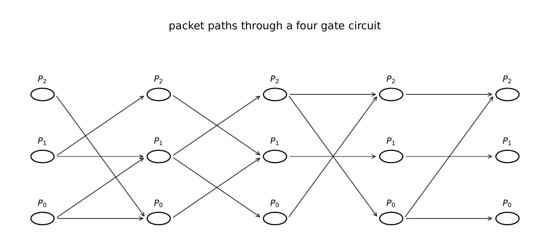
Text description
Columns of three packet nodes represent successive gate stages. Links join permitted transfers between columns, while missing links represent forbidden transfers. A circuit block is obtained by coherently summing its surviving paths.
Example II.4.6: Bell circuit
Starting from \({\left|00\right\rangle}\), apply a Hadamard gate to the first qubit and then a controlled NOT gate. The final state is
It lies in the even parity packet. The intermediate state has one even and one odd computational contribution, so the final even amplitude is reconstructed by more than one packet path.
Visual guide: Track the Bell state through the circuit · Permalink · Source line 508
II.5 Symmetry resolved dynamics and leakage
On this page · Permalink · Source line 516
Let \(H=H^*\) and let \((P_a)_{a\in I}\) be a complete orthogonal packet system.
Theorem II.5.1: Exact invariant packets
The following conditions are equivalent:
The Hamiltonian commutes with each projector: \([H,P_a]=0\) for every \(a\).
Transfer blocks between distinct packets vanish: \(P_bHP_a=0\) whenever \(a\neq b\).
Every packet \(P_a{\mathcal H}\) is invariant under \({\mathrm e}^{-{\mathrm i} tH}\) for every real \(t\).
When they hold,
and
Read proof · Visual guide: A symmetry reveals blocks, not approximations · Read statement and proof side by side · Permalink · Source line 520 · Claim record · Lean coverage · Code · Worked examples
Proof of Theorem II.5.1
Commutation is equivalent to vanishing of every off diagonal block. The same block decomposition passes to polynomials in \(H\), then to the exponential by norm convergence. Invariance of every packet implies invariance under both \({\mathrm e}^{-{\mathrm i} tH}\) and its adjoint. Differentiation at \(t=0\) gives commutation with \(H\).
Back to statement · Read statement and proof side by side · Permalink · Source line 537 · Claim record · Lean coverage · Code · Worked examples
Fix one packet projector \(P\) and set \(Q=I-P\).
Lemma II.5.2: Off diagonal norm
For self adjoint \(H\),
Read proof · Read statement and proof side by side · Permalink · Source line 543 · Claim record · Lean coverage · Code · Worked examples
Proof of Lemma II.5.2
Relative to \(P{\mathcal H}\oplus Q{\mathcal H}\),
Its square has diagonal blocks \(-PHQHP\) and \(-QHPHQ\). The norm is therefore the largest singular value of \(QHP\).
Back to statement · Read statement and proof side by side · Permalink · Source line 550 · Claim record · Lean coverage · Code · Worked examples
Theorem II.5.3: Fixed packet leakage
For every real \(t\),
Read proof · Visual guide: Quantify the amplitude that escapes · Read statement and proof side by side · Permalink · Source line 563 · Claim record · Lean coverage · Code · Worked examples
Proof of Theorem II.5.3
Let
The propagator generated by \(H_{\rm d}\) preserves \(P{\mathcal H}\) and \(Q{\mathcal H}\). Duhamel's formula relative to \(H_{\rm d}\) gives
Since \(H_{\rm o}P=QHP\) and both propagators are unitary, the norm is at most \({\left\lvert t\right\rvert}{\left\lVert QHP\right\rVert}\). Use Lemma II.5.2 for the last equality.
Back to statement · Read statement and proof side by side · Permalink · Source line 574 · Claim record · Lean coverage · Code · Worked examples
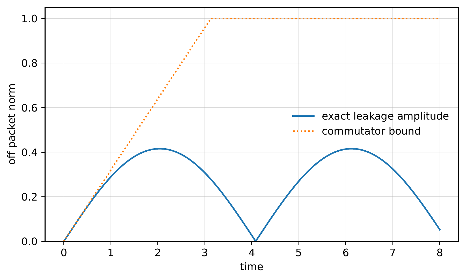
Text description
The exact leakage amplitude oscillates over the time interval. The dotted commutator envelope rises linearly and then saturates at one. The exact curve remains below that envelope in the displayed model.
Corollary II.5.4: Leakage probability
If \(\psi\in P{\mathcal H}\) is a unit vector, then
Read proof · Visual guide: Quantify the amplitude that escapes · Read statement and proof side by side · Permalink · Source line 600 · Claim record · Lean coverage · Code · Worked examples
Proof of Corollary II.5.4
Apply Theorem II.5.3 to the unit vector, then square the resulting nonnegative bound.
Back to statement · Read statement and proof side by side · Permalink · Source line 609 · Claim record · Lean coverage · Code · Worked examples
II.6 Moving packets and geometric transport
On this page · Permalink · Source line 613
Let \((P_a(t))_{a\in I}\) be a twice continuously differentiable family of complete orthogonal packet systems on a finite dimensional Hilbert space.
Theorem II.6.1: Canonical packet connection
Define
Then
and
for every \(a\).
Read proof · Visual guide: Differentiate the subspace itself · Read statement and proof side by side · Permalink · Source line 617 · Claim record · Lean coverage · Code · Worked examples
Proof of Theorem II.6.1
Differentiating \(P_a^2=P_a\) gives
Summing over \(a\) and using \(\sum_a\dot P_a=0\) yields
This proves skew adjointness. For fixed \(b\),
Differentiating \(P_bP_a=0\) for \(a\neq b\) gives
Hence
Subtracting gives \([K,P_b]=\dot P_b\).
Back to statement · Read statement and proof side by side · Permalink · Source line 635 · Claim record · Lean coverage · Code · Worked examples
Theorem II.6.2: Exact Kato transport
Let \(W(t)\) solve
Then \(W(t)\) is unitary and
for every packet \(a\).
Read proof · Visual guide: Differentiate the subspace itself · Read statement and proof side by side · Permalink · Source line 659 · Claim record · Lean coverage · Code · Worked examples
Proof of Theorem II.6.2
Skew adjointness gives
Thus \(W(t)\) is unitary. Next,
The expression equals \(P_a(0)\) at \(t=0\), which proves the intertwining identity.
Back to statement · Read statement and proof side by side · Permalink · Source line 673 · Claim record · Lean coverage · Code · Worked examples
Theorem II.6.3: Moving frame Hamiltonian
Let \(U(t)\) solve
where \(H(t)=H(t)^*\) is continuous on the compact time interval under consideration. Set
Then
where
The moving frame Hamiltonian is self adjoint.
Read proof · Visual guide: A moving frame creates a connection term · Read statement and proof side by side · Permalink · Source line 692 · Claim record · Lean coverage · Code · Worked examples
Proof of Theorem II.6.3
Differentiate \(V=W^*U\). Since \(\dot W=KW\) and \(K^*=-K\),
Substitution gives the equation. The first term in \(H_{\rm mov}\) is self adjoint. The operator \(-{\mathrm i} W^*\dot W\) is self adjoint because \(W^*\dot W\) is skew adjoint.
Back to statement · Read statement and proof side by side · Permalink · Source line 718 · Claim record · Lean coverage · Code · Worked examples
Theorem II.6.4: Moving packet leakage
Fix a packet \(P(t)=P_a(t)\) and put \(Q(t)=I-P(t)\). For \(0\leq t\leq T\),
In particular, the physical evolution follows the moving packet exactly on \([0,T]\) when the displayed off packet block vanishes for every time in that interval.
Read proof · Read statement and proof side by side · Permalink · Source line 726 · Claim record · Lean coverage · Code · Worked examples
Proof of Theorem II.6.4
In the Kato frame, \(P(0)\) is fixed and
Apply the time dependent version of the Duhamel argument in Theorem II.5.3 to \(H_{\rm mov}(t)\). The off diagonal block is
Unitary conjugation preserves the norm.
Back to statement · Read statement and proof side by side · Permalink · Source line 738 · Claim record · Lean coverage · Code · Worked examples
The exact coupling test therefore includes the geometric term. Even if the Hamiltonian is diagonal in the packet decomposition at every fixed time, its evolution can fail to follow a packet whose range rotates.
II.6.1 Discrete packet transport
On this page · Permalink · Source line 756
Let \((P_a)\) and \((Q_a)\) be two complete packet systems with the same index set. Define
Theorem II.6.5: Direct packet rotation
Assume
Then \(S({\mathcal Q},{\mathcal P})\) is invertible. Its unitary polar factor
satisfies
for every \(a\).
Read proof · Visual guide: Rotate whole packets by a polar factor · Read statement and proof side by side · Permalink · Source line 763 · Claim record · Lean coverage · Code · Worked examples
Proof of Theorem II.6.5
The norm condition gives invertibility by the Neumann series. The identity
shows that \(S^*S\) commutes with every \(P_a\). Its inverse square root also commutes with every \(P_a\). Hence
The polar factor is unitary because \(S\) is invertible.
Back to statement · Read statement and proof side by side · Permalink · Source line 783 · Claim record · Lean coverage · Code · Worked examples
Theorem II.6.6: Convergence of short packet rotations
Let \((P_a(t))\) be twice continuously differentiable on \([0,T]\). For a partition
let
For sufficiently fine partitions the factors are defined, and
for a constant depending on the packet path but not on the partition. Here the size of the partition is measured by its mesh, which is the length of its largest subinterval.
Read proof · Visual guide: Rotate whole packets by a polar factor · Read statement and proof side by side · Permalink · Source line 798 · Claim record · Lean coverage · Code · Worked examples
Proof of Theorem II.6.6
Taylor expansion gives
uniformly on \([0,T]\). Since \(K(t)^*=-K(t)\),
so the polar factor satisfies
This gives a first order approximation to \(\dot W=KW\) over a single time step. A telescoping product estimate over the partition gives a total error bounded by a constant times \(\sum_j(t_{j+1}-t_j)^2\), which is at most \(T{\left\lvert\pi\right\rvert}\).
Back to statement · Read statement and proof side by side · Permalink · Source line 820 · Claim record · Lean coverage · Code · Worked examples
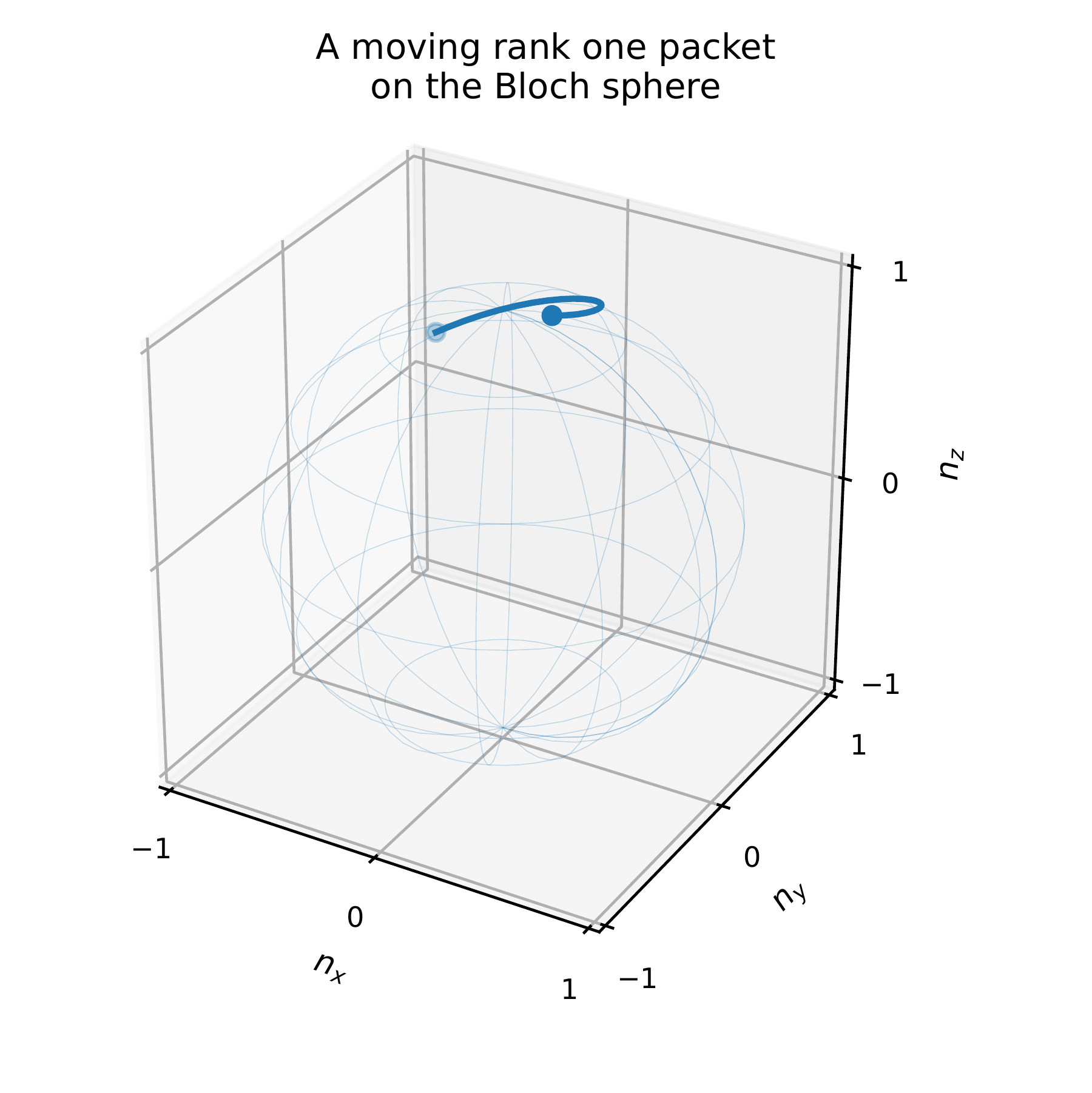
Text description
A three-dimensional Bloch-sphere coordinate plot shows a curved path near the upper part of the sphere. It illustrates transport of a one-dimensional range. The Kato construction follows that range without choosing an eigenvector phase.
II.6.2 Local frames and curvature
On this page · Permalink · Source line 848
Let \(P(x)\) be a smooth rank \(r\) orthogonal projector over a parameter manifold. Choose a local isometry
Theorem II.6.7: Nonabelian packet connection
The one form with matrix values
is skew adjoint. Under a frame change \(V'=VG\), where \(G(x)\in U(r)\),
Its curvature
satisfies
Read proof · Visual guide: A chart failure is not a singular fiber · Visual guide: Curvature measures a local area response · Read statement and proof side by side · Permalink · Source line 857 · Claim record · Lean coverage · Code · Worked examples
Proof of Theorem II.6.7
Differentiate \(V^*V=I\) to obtain \({\mathcal A}^*=-{\mathcal A}\). The gauge transformation law follows by differentiating \(VG\). Since \(P=VV^*\) and \((I-P){\,\mathrm d} V={\,\mathrm d} P\,V\), direct expansion gives
Back to statement · Read statement and proof side by side · Permalink · Source line 878 · Claim record · Lean coverage · Code · Worked examples
Corollary II.6.8: Bloch sphere curvature
Let
where
With the convention
one has
and
Read proof · Visual guide: Curvature measures a local area response · Read statement and proof side by side · Permalink · Source line 889 · Claim record · Lean coverage · Code · Worked examples
Proof of Corollary II.6.8
The Pauli identity
gives
Integrating the displayed curvature over the sphere and applying the stated normalization gives one.
Back to statement · Read statement and proof side by side · Permalink · Source line 918 · Claim record · Lean coverage · Code · Worked examples
II.7 Operator packets, measurements, and quantum channels
On this page · Visual guide: Three objects, three questions · Permalink · Source line 936
Density matrices and observables carry both an input packet and an output packet. Equip \({\operatorname{End}}({\mathcal H})\) with the Hilbert Schmidt inner product
Definition II.7.1: Two sided operator packet
For a complete orthogonal family \((P_a)\), define
The range
is the operator packet with output address \(a\) and input address \(b\).
Visual guide: The objects on the page · Permalink · Source line 943 · Claim record · Lean coverage · Code · Worked examples
Theorem II.7.2: Complete operator packet system
The superoperators \(({\mathcal P}_{ab})_{a,b\in I}\) are mutually orthogonal projections on Hilbert Schmidt operator space. They satisfy
and
Read proof · Visual guide: Which coherence can a measurement see? · Read statement and proof side by side · Permalink · Source line 955 · Claim record · Lean coverage · Code · Worked examples
Proof of Theorem II.7.2
Idempotence and completeness follow from the projector identities. For Hilbert Schmidt orthogonality,
Since the packets are orthogonal and sum to the original operator, their squared norms add to its squared norm.
Back to statement · Read statement and proof side by side · Permalink · Source line 968 · Claim record · Lean coverage · Code · Worked examples
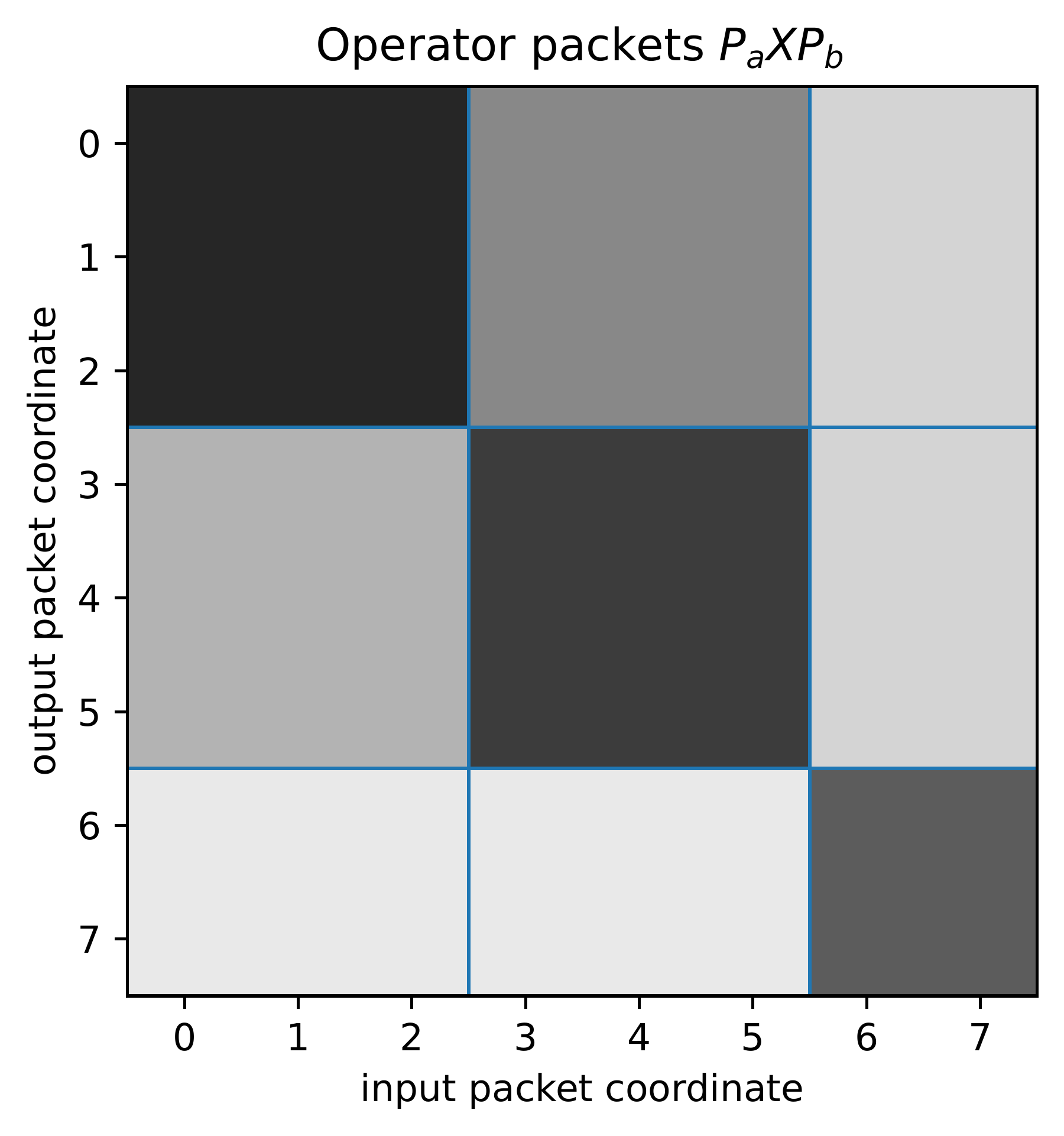
Text description
Rows and columns are grouped into three packet address ranges, producing a three-by-three array of shaded blocks. A block has an output packet address and an input packet address. Diagonal blocks contain within-packet information; off-diagonal blocks contain cross-packet coherence.
Definition II.7.3: Packet dephasing
The packet dephasing map is
Permalink · Source line 990 · Claim record · Lean coverage · Code · Worked examples
Theorem II.7.4: Dephasing as conditional expectation
The map \({\mathcal D}_{{\mathcal P}}\) is completely positive, trace preserving, unital, and idempotent. It is the Hilbert Schmidt orthogonal projection onto the block diagonal algebra
In particular,
Read proof · Visual guide: Which coherence can a measurement see? · Visual guide: One calculation of transfer to the opposite site · Read statement and proof side by side · Permalink · Source line 997 · Claim record · Lean coverage · Code · Worked examples
Proof of Theorem II.7.4
The projectors \(P_a\) form a Kraus family because \(\sum_aP_a^*P_a=I\). Thus the map is completely positive and trace preserving. It is unital for the same reason. Orthogonality and idempotence follow from Theorem II.7.2. Its range is the sum of the diagonal operator packets. This is exactly the commutant of the projector family.
Back to statement · Read statement and proof side by side · Permalink · Source line 1012 · Claim record · Lean coverage · Code · Worked examples
Corollary II.7.5: Block diagonal measurement invariance
Let \((E_k)\) be a positive operator valued measurement, and suppose
for every \(k\). Then every density matrix \(\rho\) satisfies
Read proof · Visual guide: Which coherence can a measurement see? · Read statement and proof side by side · Permalink · Source line 1016 · Claim record · Lean coverage · Code · Worked examples
Proof of Corollary II.7.5
Since \({\mathcal D}_{{\mathcal P}}\) is self adjoint for the Hilbert Schmidt inner product,
Back to statement · Read statement and proof side by side · Permalink · Source line 1029 · Claim record · Lean coverage · Code · Worked examples
II.7.1 Channel superblocks
On this page · Permalink · Source line 1040
Let \(\Phi:{\operatorname{End}}({\mathcal H}_X)\to{\operatorname{End}}({\mathcal H}_Y)\) be linear. Choose packet systems \((P_a)\) on \({\mathcal H}_X\) and \((Q_c)\) on \({\mathcal H}_Y\). Define
Theorem II.7.6: Exact channel block calculus
Every linear map has the exact reconstruction
If \(\Psi:{\operatorname{End}}({\mathcal H}_Y)\to{\operatorname{End}}({\mathcal H}_Z)\), then
Read proof · Visual guide: A channel acts on four matrix entries · Read statement and proof side by side · Permalink · Source line 1049 · Claim record · Lean coverage · Code · Worked examples
Proof of Theorem II.7.6
Insert the complete operator packet resolutions before and after \(\Phi\). For composition, insert the middle resolution between \(\Psi\) and \(\Phi\) and collect the output and input packets.
Back to statement · Read statement and proof side by side · Permalink · Source line 1063 · Claim record · Lean coverage · Code · Worked examples
Standard fact II.7.7: Finite Kraus and Choi criteria
A linear map \(\Phi:M_n({\mathbb C})\to M_m({\mathbb C})\) is completely positive exactly when it has a Kraus representation
It is trace preserving exactly when
Equivalently, its Choi matrix
is positive, and trace preservation is
Visual guide: An ancilla tests more than positivity · Permalink · Source line 1067 · Claim record · Lean coverage · Code · Worked examples
These finite criteria are classical [Stinespring1955], [Choi1975], [Kraus1983], [Watrous2018].
II.7.2 Covariance and coherence order
On this page · Permalink · Source line 1090
Let \(S\) be unitary and \(N\ge1\) an integer with \(S^N=I\), and define the conjugation action
Theorem II.7.8: Coherence order projectors
For \(q\in{\mathbb Z}/N{\mathbb Z}\), define
Then the \({\mathcal L}_q\) form a complete orthogonal packet system on Hilbert Schmidt operator space. Their ranges are the operators satisfying
If \(P_j\) are the state charge projectors, then
Read proof · Visual guide: Coherence order survives a covariant channel · Read statement and proof side by side · Permalink · Source line 1097 · Claim record · Lean coverage · Code · Worked examples
Proof of Theorem II.7.8
Apply the cyclic character projector formula to the unitary representation \({\operatorname{Ad}}_S\) on operator space. The last identity follows from Theorem II.3.5 applied to each operator packet.
Back to statement · Read statement and proof side by side · Permalink · Source line 1118 · Claim record · Lean coverage · Code · Worked examples
Theorem II.7.9: Covariant channels preserve coherence order
Suppose
for every \(X\). Then
for every \(q\). Thus \(\Phi\) cannot mix distinct coherence orders.
Read proof · Read statement and proof side by side · Permalink · Source line 1122 · Claim record · Lean coverage · Code · Worked examples
Proof of Theorem II.7.9
The covariance identity says that \(\Phi\) commutes with every power of \({\operatorname{Ad}}_S\). It therefore commutes with each finite character average \({\mathcal L}_q\).
Back to statement · Read statement and proof side by side · Permalink · Source line 1134 · Claim record · Lean coverage · Code · Worked examples
Theorem II.7.10: Choi symmetry criterion
Let \(U:G\to{\mathcal U}({\mathcal H})\) be a finite group representation. A channel \(\Phi\) is covariant,
if and only if
for every \(g\in G\).
Read proof · Visual guide: Coherence order survives a covariant channel · Read statement and proof side by side · Permalink · Source line 1138 · Claim record · Lean coverage · Code · Worked examples
Proof of Theorem II.7.10
Let
Then
The vector \(\Omega\) is invariant under \(U\otimes\overline U\). Covariance therefore implies the displayed Choi invariance. Conversely, the displayed transformation is the Choi matrix of
The Choi correspondence is injective, so invariance implies that this map equals \(\Phi\), which is covariance.
Back to statement · Read statement and proof side by side · Permalink · Source line 1156 · Claim record · Lean coverage · Code · Worked examples
Corollary II.7.11: Choi packet decomposition
The Choi matrix of a covariant channel is block diagonal with respect to the isotypic decomposition of \(U\otimes\overline U\).
Read proof · Read statement and proof side by side · Permalink · Source line 1172 · Claim record · Lean coverage · Code · Worked examples
Proof of Corollary II.7.11
Apply Theorem II.3.1 to the representation \(U\otimes\overline U\) and use Theorem II.7.10.
Back to statement · Read statement and proof side by side · Permalink · Source line 1176 · Claim record · Lean coverage · Code · Worked examples
Example II.7.12: Amplitude damping
For \(0\leq\gamma\leq1\), let
The channel
is trace preserving. It sends the off diagonal packet \({\left|0\right\rangle}{\left\langle1\right|}\) to \(\sqrt{1-\gamma}{\left|0\right\rangle}{\left\langle1\right|}\), while the excited population transfers partly into the ground population.
Visual guide: A channel acts on four matrix entries · Permalink · Source line 1180
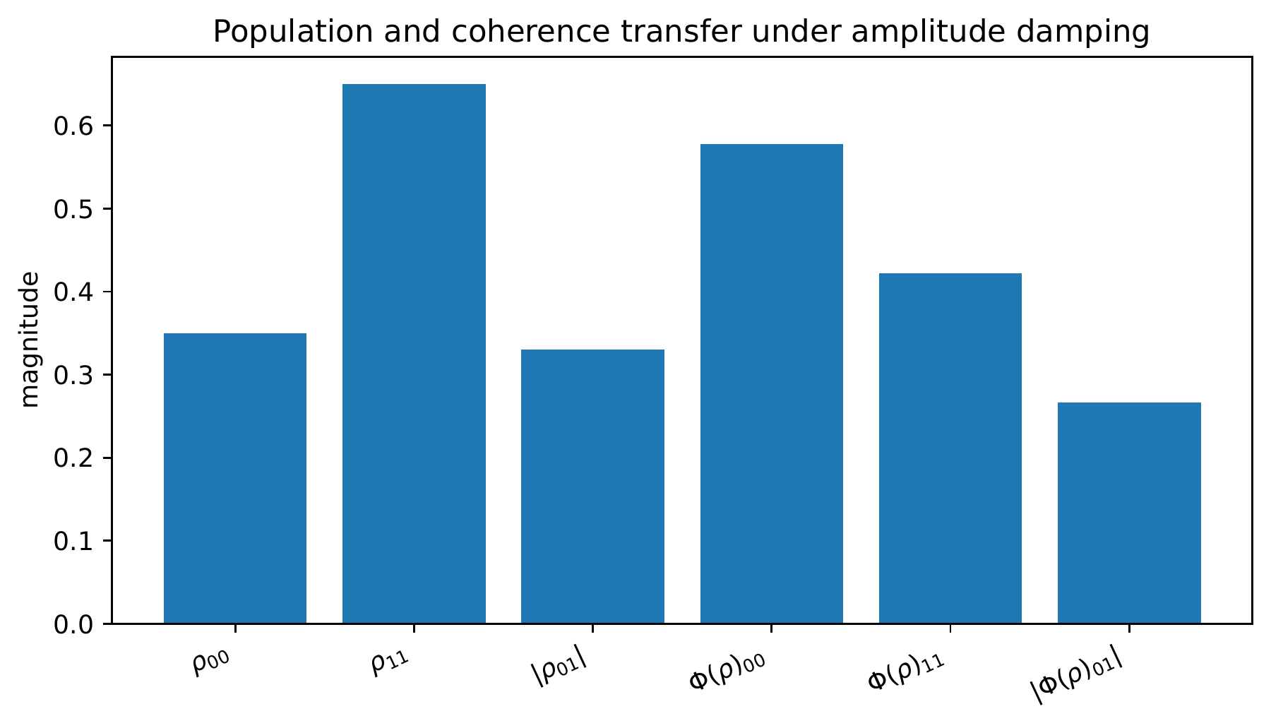
Text description
Six bars compare the two input populations and input coherence magnitude with their three channel outputs. The ground population increases, the excited population decreases, and the coherence magnitude contracts. The bars depict one finite density-matrix example.
II.7.3 Quantum dynamical semigroups
On this page · Permalink · Source line 1210
Standard fact II.7.13: Finite Lindblad generator
A norm continuous semigroup of completely positive trace preserving maps on a finite matrix algebra, in the Schrödinger picture, has a generator of the form
where \(H=H^*\). Conversely, every operator of this form generates a completely positive trace preserving semigroup [Lindblad1976].
Permalink · Source line 1212 · Claim record · Lean coverage · Code · Worked examples
Theorem II.7.14: Charge preservation by a Lindblad generator
Let \(S\) be unitary and \(N\ge1\) an integer with \(S^N=I\). Assume
and, for every jump operator, there is a charge \(q_r\) such that
Then the Lindblad generator \({\mathcal G}\) preserves every coherence order:
The quantum dynamical semigroup \({\mathrm e}^{t{\mathcal G}}\) has the same property.
Read proof · Visual guide: Coherence order survives a covariant channel · Read statement and proof side by side · Permalink · Source line 1231 · Claim record · Lean coverage · Code · Worked examples
Proof of Theorem II.7.14
Let \(X\) have coherence order \(p\). The Hamiltonian commutator has order \(p\) because \(H\) has charge zero. The jump term \(L_rXL_r^*\) has charge
Also \(L_r^*L_r\) has charge zero, so both anticommutator terms have charge \(p\). Thus \({\mathcal G}\) preserves \({\operatorname{Ran}}{\mathcal L}_p\). The exponential series then shows that \({\mathrm e}^{t{\mathcal G}}\) preserves the same packets.
Back to statement · Read statement and proof side by side · Permalink · Source line 1247 · Claim record · Lean coverage · Code · Worked examples
Corollary II.7.15: Independent coherence evolution
Under the hypotheses of Theorem II.7.14, each coherence component of an initial operator evolves within its own order. In particular, a density matrix in the zero order sector remains in that sector.
Read proof · Read statement and proof side by side · Permalink · Source line 1255 · Claim record · Lean coverage · Code · Worked examples
Proof of Corollary II.7.15
Decompose the initial operator by Theorem II.7.8 and apply the invariant packet statement to each component.
Back to statement · Read statement and proof side by side · Permalink · Source line 1259 · Claim record · Lean coverage · Code · Worked examples
Preservation of coherence order does not by itself give a closed classical Markov chain for the packet populations. Such scalar population equations require additional isotropy within each packet.
II.8 Quantum error correction as a compression obstruction
On this page · Permalink · Source line 1265
Let \(P\) be the orthogonal projector onto a code space
The compression of \(A\in{\operatorname{End}}({\mathcal H})\) to the code is \(PAP\in{\operatorname{End}}({\mathcal C})\). The zero code has only the zero supported operator and no normalized code state. Part III treats that branch in the mathematical completion.
Definition II.8.1: Code compression obstruction
Let
be the quotient map. Define
Equivalently, one may use the traceless representative
Permalink · Source line 1275 · Claim record · Lean coverage · Code · Worked examples
The class vanishes exactly when \(A\) acts as a scalar after compression to the code. Such an operator cannot distinguish normalized code vectors by expectation value.
Exact correction of an error span means that one completely positive trace preserving recovery \({\mathcal R}\) satisfies \({\mathcal R}(F\rho F^*)=q_F\rho\) for every \(F\) in that span and every code-supported matrix \(\rho\), with a nonnegative scalar \(q_F\) depending on \(F\) but not on the logical input. For every normalized channel with Kraus operators in the same span, the same recovery restores the code input with total scalar one. Individual unnormalized errors are not required to have unit recovery weight.
Theorem II.8.2: Knill Laflamme as obstruction vanishing
Let \(E_1,\ldots,E_r\) be an error family. The code \({\mathcal C}\) corrects their linear span exactly if and only if
for all \(a,b\). Equivalently, there is a matrix \(c=(c_{ab})\) such that
for all \(a,b\).
Read proof · Visual guide: Find the error without reading the logical state · Visual guide: An unchanged syndrome can hide a logical error · Read statement and proof side by side · Permalink · Source line 1297 · Claim record · Lean coverage · Code · Worked examples
Proof of Theorem II.8.2
The equivalence between the quotient statement and the scalar compression identity is immediate from the definition. The latter identity is the finite Knill Laflamme criterion [KnillLaflamme1997], [SchumacherNielsen1996].
Back to statement · Read statement and proof side by side · Permalink · Source line 1309 · Claim record · Lean coverage · Code · Worked examples
The next result turns the scalar compression identities into a family of orthogonal syndrome packets. Those packets provide the coordinates used by the recovery map.
Theorem II.8.3: Orthogonal syndrome construction
Assume the Knill Laflamme identities. Then the coefficient matrix \(c\) is positive semidefinite. Choose a unitary matrix \(W\) such that
and define
For every \(j\) with \(\lambda_j>0\), the operator
is an isometry from the code into \({\mathcal H}\). Its range projector
is a syndrome packet, and the nonzero \(Q_j\) are pairwise orthogonal.
Read proof · Visual guide: Null Gram directions are removed before recovery · Read statement and proof side by side · Permalink · Source line 1315 · Claim record · Lean coverage · Code · Worked examples
Proof of Theorem II.8.3
For \(z\in{\mathbb C}^r\), let \(F_z=\sum_az_aE_a\). Then
so \(c\geq0\). The unitary change of error coordinates gives
Thus
Each \(V_j\) is an isometry on \(P{\mathcal H}\), and distinct ranges are orthogonal. Their range projectors are therefore pairwise orthogonal.
Back to statement · Read statement and proof side by side · Permalink · Source line 1337 · Claim record · Lean coverage · Code · Worked examples
Theorem II.8.4: Exact recovery on the error span
Under the hypotheses of Theorem II.8.3, define on the syndrome support
the completely positive map
It extends to a quantum channel \({\mathcal R}\) on \({\operatorname{End}}({\mathcal H})\). If
is trace preserving on code states, then
for every density matrix \(\rho=P\rho P\).
Read proof · Visual guide: Find the error without reading the logical state · Visual guide: Null Gram directions are removed before recovery · Read statement and proof side by side · Permalink · Source line 1355 · Claim record · Lean coverage · Code · Worked examples
Proof of Theorem II.8.4
The map \({\mathcal R}_0\) is completely positive. It is trace preserving on operators supported in \(Q{\mathcal H}\) because
Fix a code state \(\rho_0\) and write \(Q^\perp=I-Q\). Then
is completely positive and trace preserving. It extends \({\mathcal R}_0\) on operators supported in \(Q{\mathcal H}\).
Unitary mixing of a Kraus family does not change the channel, so
Recovery gives
Trace preservation on a code state implies \(\sum_j\lambda_j=1\).
Back to statement · Read statement and proof side by side · Permalink · Source line 1378 · Claim record · Lean coverage · Code · Worked examples
Corollary II.8.5: Syndrome measurement preserves logical information
For a channel trace preserving on code states as in the preceding theorem, the completed projective measurement consisting of \((Q_j)_{\lambda_j>0}\) and \(I-\sum_{\lambda_j>0}Q_j\) identifies the orthogonal error syndrome without resolving the encoded state inside the code. The complement outcome has probability zero on the corrupted code state.
Read proof · Read statement and proof side by side · Permalink · Source line 1413 · Claim record · Lean coverage · Code · Worked examples
Proof of Corollary II.8.5
On syndrome \(j\), the encoded state is carried by the isometry \(V_j\). The outcome probability is \(\lambda_j\), independent of the normalized code state, while the postmeasurement state is \(V_j\rho V_j^*\).
Back to statement · Read statement and proof side by side · Permalink · Source line 1417 · Claim record · Lean coverage · Code · Worked examples
Definition II.8.6: Approximate Knill Laflamme defect
For a finite error family, define the following defect. When the family is empty, assign the maximum the value zero.
Visual guide: An approximate defect has a precise norm meaning · Permalink · Source line 1421 · Claim record · Lean coverage · Code · Worked examples
Proposition II.8.7: Meaning of the approximate defect
For each pair \((a,b)\), choose a minimizing scalar \(c_{ab}\). For unit code vectors \(\psi,\phi\),
Thus \(\varepsilon_{\rm KL}\) controls the deviation of error overlaps from their scalar code form.
Read proof · Visual guide: An unchanged syndrome can hide a logical error · Visual guide: An approximate defect has a precise norm meaning · Read statement and proof side by side · Permalink · Source line 1432 · Claim record · Lean coverage · Code · Worked examples
Proof of Proposition II.8.7
The left side is
which is bounded by the operator norm.
Back to statement · Read statement and proof side by side · Permalink · Source line 1445 · Claim record · Lean coverage · Code · Worked examples
No recovery fidelity estimate is inferred from this norm alone. Approximate error correction requires a separate continuity theorem and a declared channel metric.
Example II.8.8: Three qubit repetition code
Let
and take the errors
Their images of the code are four pairwise orthogonal two dimensional syndrome packets whose sum is the full eight dimensional Hilbert space.
Visual guide: Find the error without reading the logical state · Permalink · Source line 1457
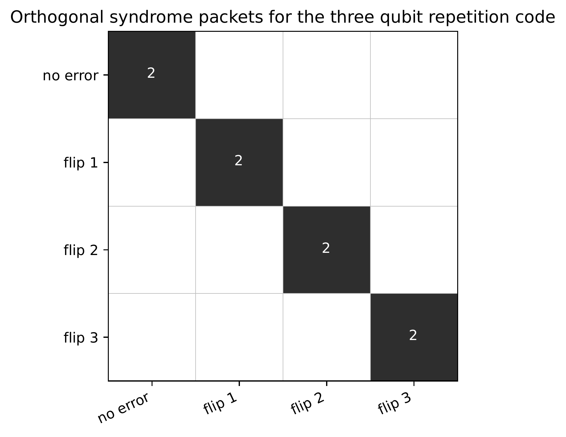
Text description
A four-by-four schematic has one marked diagonal square for each error syndrome. Every marked square is labeled dimension two. Distinct syndrome packets are orthogonal and each retains the full logical state.
Standard fact II.8.9: Correctable observable algebras
Let \(\Phi\) be a finite completely positive trace preserving channel with Kraus operators \((E_a)\). A finite dimensional unital star subalgebra \({\mathcal M}\subseteq P{\operatorname{End}}({\mathcal H})P\) is correctable when a completely positive trace preserving recovery \({\mathcal R}\) satisfies \(P(\Phi^*\circ{\mathcal R}^*)(X)P=X\) for every \(X\in{\mathcal M}\), where stars on maps denote Heisenberg adjoints. This holds exactly when every compressed product \(PE_a^*E_bP\) belongs to the commutant \({\mathcal M}'\) on the code. The scalar code criterion is the special case \({\mathcal M}=P{\operatorname{End}}({\mathcal H})P\) [BenyKempfKribs2007].
Permalink · Source line 1484 · Claim record · Lean coverage · Code · Worked examples
II.9 Feshbach effective dynamics and hidden packet memory
On this page · Visual guide: Three objects, three questions · Permalink · Source line 1488
Let \(P\) be an orthogonal projector, put \(Q=I-P\), and write a self adjoint Hamiltonian as
relative to \(P{\mathcal H}\oplus Q{\mathcal H}\).
Definition II.9.1: Feshbach map and self energy
For \(z\notin{\operatorname{Spec}} D\), define
and
Permalink · Source line 1500 · Claim record · Lean coverage · Code · Worked examples
Theorem II.9.2: Exact projected resolvent
If \(z\notin{\operatorname{Spec}} D\) and \(F_P(z)\) is invertible, then
as an operator on \(P{\mathcal H}\).
Read proof · Visual guide: Hidden states return as spectral dependence · Read statement and proof side by side · Permalink · Source line 1511 · Claim record · Lean coverage · Code · Worked examples
Proof of Theorem II.9.2
The lower right block of \(z-H\) is \(z-D\). Block Gaussian elimination gives
Invert the factors. The retained resolvent is the block in the upper left corner of the resulting inverse.
Back to statement · Read statement and proof side by side · Permalink · Source line 1519 · Claim record · Lean coverage · Code · Worked examples
Theorem II.9.3: Spectral equivalence
Let \(z\notin{\operatorname{Spec}} D\). Then
The map
is an isomorphism from \({\operatorname{Ker}} F_P(z)\) onto \({\operatorname{Ker}}(z-H)\).
Read proof · Visual guide: Hidden states return as spectral dependence · Read statement and proof side by side · Permalink · Source line 1540 · Claim record · Lean coverage · Code · Worked examples
Proof of Theorem II.9.3
The equation \((z-H)(x,y)^{\mathsf T}=0\) is
The second equation gives \(y=(z-D)^{-1}B^*x\). Substitution into the first gives \(F_P(z)x=0\). The construction is reversible.
Back to statement · Read statement and proof side by side · Permalink · Source line 1558 · Claim record · Lean coverage · Code · Worked examples
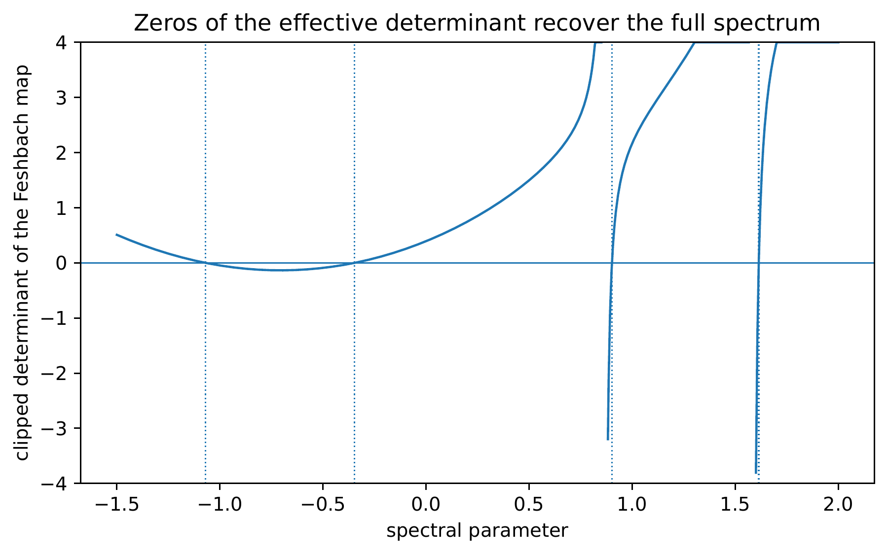
Text description
The plot shows the clipped Feshbach determinant as a function of spectral parameter. Vertical reference lines mark full-Hamiltonian eigenvalues, while sharp features occur near the hidden spectrum. The stated correspondence excludes the hidden-spectrum poles.
Theorem II.9.4: Upper half plane sign
If \(\operatorname{Im}z>0\), then
Thus \(-\Sigma\) is an operator valued Herglotz function.
Read proof · Visual guide: Control the hidden spectral response · Read statement and proof side by side · Permalink · Source line 1575 · Claim record · Lean coverage · Code · Worked examples
Proof of Theorem II.9.4
For \(R(z)=(z-D)^{-1}\), the resolvent identity gives
Divide by \(2{\mathrm i}\), then multiply the result on the left by \(B\) and on the right by \(B^*\).
Back to statement · Read statement and proof side by side · Permalink · Source line 1587 · Claim record · Lean coverage · Code · Worked examples
Proposition II.9.5: Uniform self energy bounds
Let
Then
and
For real \(E,E'\) in an interval at distance at least \(\delta\) from \({\operatorname{Spec}} D\),
Read proof · Visual guide: Control the hidden spectral response · Read statement and proof side by side · Permalink · Source line 1596 · Claim record · Lean coverage · Code · Worked examples
Proof of Proposition II.9.5
The self adjoint resolvent satisfies
Differentiate the resolvent to obtain
Taking operator norms gives the first two estimates. Applying the derivative bound along the real interval gives the final mean value estimate.
Back to statement · Read statement and proof side by side · Permalink · Source line 1619 · Claim record · Lean coverage · Code · Worked examples
Proposition II.9.6: Low energy expansion
Assume \(D\) is invertible and \({\left\lvert z\right\rvert}{\left\lVert D^{-1}\right\rVert}<1\). Then
with norm convergence. In particular,
Read proof · Read statement and proof side by side · Permalink · Source line 1631 · Claim record · Lean coverage · Code · Worked examples
Proof of Proposition II.9.6
Write
and multiply on the left by \(B\) and on the right by \(B^*\).
Back to statement · Read statement and proof side by side · Permalink · Source line 1647 · Claim record · Lean coverage · Code · Worked examples
Proposition II.9.7: Bare truncation error identity
If both \(F_P(z)\) and \(z-A\) are invertible, then
Read proof · Read statement and proof side by side · Permalink · Source line 1657 · Claim record · Lean coverage · Code · Worked examples
Proof of Proposition II.9.7
Use the inverse difference identity
with \(X=F_P(z)\) and \(Y=z-A\).
Back to statement · Read statement and proof side by side · Permalink · Source line 1666 · Claim record · Lean coverage · Code · Worked examples
II.9.1 Time memory
On this page · Permalink · Source line 1674
Write a Schrödinger state as \(\psi=x+y\), where \(x=P\psi\) and \(y=Q\psi\).
Theorem II.9.8: Exact retained memory equation
The retained coordinate satisfies
where
For \(\operatorname{Re}s>0\),
Read proof · Visual guide: The smaller system remembers the discarded one · Read statement and proof side by side · Permalink · Source line 1678 · Claim record · Lean coverage · Code · Worked examples
Proof of Theorem II.9.8
The hidden equation is
Variation of constants gives
Substitute into \({\mathrm i}\dot x=Ax+By\). The Laplace formula follows by diagonalizing \(D\) or integrating the norm convergent finite dimensional exponential.
Back to statement · Read statement and proof side by side · Permalink · Source line 1699 · Claim record · Lean coverage · Code · Worked examples
Theorem II.9.9: Positive definite quantum memory
The kernel \(K(t-s)\) is positive definite. For times \(t_1,\ldots,t_m\) and retained vectors \(v_1,\ldots,v_m\),
Read proof · Visual guide: Memory positivity is a Gram identity · Read statement and proof side by side · Permalink · Source line 1712 · Claim record · Lean coverage · Code · Worked examples
Proof of Theorem II.9.9
Set
Then
Back to statement · Read statement and proof side by side · Permalink · Source line 1721 · Claim record · Lean coverage · Code · Worked examples
Corollary II.9.10: Finite oscillatory memory expansion
If
is the spectral decomposition of the hidden Hamiltonian, then
Every coefficient \(BQ_rB^*\) is positive semidefinite.
Read proof · Read statement and proof side by side · Permalink · Source line 1738 · Claim record · Lean coverage · Code · Worked examples
Proof of Corollary II.9.10
Inserting the spectral decomposition into the exponential gives the stated sum. The spectral projectors are positive semidefinite, so multiplication by the coupling and its adjoint preserves positivity of each coefficient.
Back to statement · Read statement and proof side by side · Permalink · Source line 1750 · Claim record · Lean coverage · Code · Worked examples
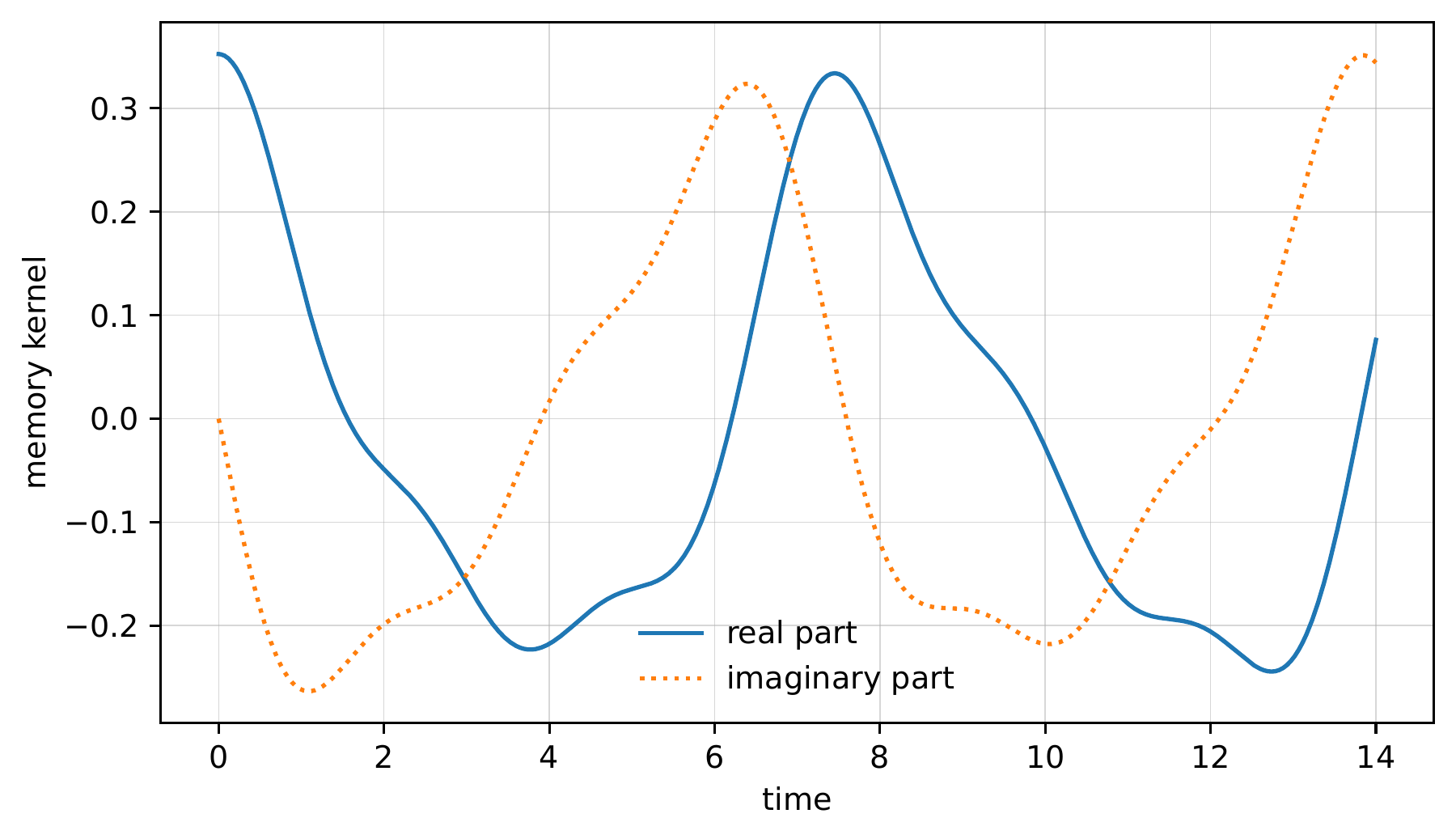
Text description
Two curves oscillate above and below zero as time increases, one for the real part and one for the imaginary part. The finite hidden spectrum produces memory, so the retained dynamics depend on earlier retained states.
Theorem II.9.11: Exact local closure criterion
Assume \(y(0)=0\). The retained equation is local and equal to
for every retained initial state exactly when \(B=0\). Equivalently, exact local closure holds exactly when the retained and hidden packets reduce \(H\).
Read proof · Visual guide: The smaller system remembers the discarded one · Visual guide: Memory positivity is a Gram identity · Read statement and proof side by side · Permalink · Source line 1761 · Claim record · Lean coverage · Code · Worked examples
Proof of Theorem II.9.11
If \(B=0\), the retained and hidden equations decouple. Conversely, suppose that every solution with \(y(0)=0\) satisfies \(x(t)={\mathrm e}^{-{\mathrm i} tA}x(0)\). The full block equation gives
while the declared local equation gives
Since this holds for every retained initial vector, \(BB^*=0\). Hence \(B=0\).
Back to statement · Read statement and proof side by side · Permalink · Source line 1769 · Claim record · Lean coverage · Code · Worked examples
II.9.2 Stability across models
On this page · Permalink · Source line 1783
Theorem II.9.12: Stability of the self energy
Let \(D=D^*\) and \(\widetilde D=\widetilde D^*\) act on one fixed hidden Hilbert space, and let \(B,\widetilde B\) map that hidden space to one fixed retained Hilbert space. Define
Assume
and
Then
Read proof · Visual guide: Control the hidden spectral response · Read statement and proof side by side · Permalink · Source line 1785 · Claim record · Lean coverage · Code · Worked examples
Proof of Theorem II.9.12
Add and subtract \(\widetilde B(z-D)^{-1}B^*\) and \(\widetilde B(z-D)^{-1}\widetilde B^*\). The first two differences give the coupling term. For the last, use
Apply the resolvent bounds.
Back to statement · Read statement and proof side by side · Permalink · Source line 1812 · Claim record · Lean coverage · Code · Worked examples
Corollary II.9.13: Uniform Feshbach control
For a family represented on fixed retained and hidden Hilbert spaces, with self adjoint hidden Hamiltonians, a common hidden spectral separation \(\delta\), and a common coupling bound \(g\), the self energies are uniformly bounded and uniformly Lipschitz on the declared spectral region. If the couplings and hidden Hamiltonians converge in norm, then the self energies converge uniformly there.
Read proof · Read statement and proof side by side · Permalink · Source line 1821 · Claim record · Lean coverage · Code · Worked examples
Proof of Corollary II.9.13
The common gap and coupling bounds allow Proposition II.9.5 and Theorem II.9.12 to be applied uniformly across the family.
Back to statement · Read statement and proof side by side · Permalink · Source line 1825 · Claim record · Lean coverage · Code · Worked examples
This result identifies hypotheses that make Feshbach control uniform in the cutoff. Whether a chosen geometric refinement tower satisfies those hypotheses remains a separate question.
II.10 Euclidean transfer and finite reflection positivity
On this page · Permalink · Source line 1831
Let \(H=H^*\) on a nonzero finite dimensional Hilbert space and let
For a lattice time step \(a>0\), define
Theorem II.10.1: Finite Euclidean transfer
The operator \(T\) is positive definite, self adjoint, and contractive. Its spectrum lies in \((0,1]\), and
for every \(n\in{\mathbb N}\).
Read proof · Visual guide: Positive transfer is not a stochastic matrix · Read statement and proof side by side · Permalink · Source line 1842 · Claim record · Lean coverage · Code · Worked examples
Proof of Theorem II.10.1
Diagonalize \(H\). Each eigenvalue of \(T\) is
and therefore lies in \((0,1]\). The power law follows from the functional calculus.
Back to statement · Read statement and proof side by side · Permalink · Source line 1850 · Claim record · Lean coverage · Code · Worked examples
Theorem II.10.2: Hamiltonian reconstruction from transfer
Let \(T\) be positive definite, self adjoint, and contractive. Then
is a nonnegative self adjoint operator and
It is the unique nonnegative self adjoint operator with \(T={\mathrm e}^{-aH_T}\).
Read proof · Visual guide: A positive transfer determines its Hamiltonian · Read statement and proof side by side · Permalink · Source line 1858 · Claim record · Lean coverage · Code · Worked examples
Proof of Theorem II.10.2
Apply the real logarithm to the positive spectrum of \(T\). The spectral calculus gives existence and the power identity. Injectivity of the scalar exponential on \([0,\infty)\) gives uniqueness.
Back to statement · Read statement and proof side by side · Permalink · Source line 1870 · Claim record · Lean coverage · Code · Worked examples
Theorem II.10.3: Finite reflection positivity
For vectors \(v_1,\ldots,v_m\in{\mathcal H}\) and nonnegative integers \(n_1,\ldots,n_m\), the matrix
is positive semidefinite. Equivalently,
for every \(c\in{\mathbb C}^m\).
Read proof · Visual guide: Positive transfer is not a stochastic matrix · Read statement and proof side by side · Permalink · Source line 1874 · Claim record · Lean coverage · Code · Worked examples
Proof of Theorem II.10.3
Since \(T\) is positive and self adjoint,
The quadratic form is the squared norm of
Back to statement · Read statement and proof side by side · Permalink · Source line 1888 · Claim record · Lean coverage · Code · Worked examples
Corollary II.10.4: Reflection positive correlators
Fix a vector \(\Omega\) and operators \(A_1,\ldots,A_m\). The matrix
is positive semidefinite.
Read proof · Read statement and proof side by side · Permalink · Source line 1901 · Claim record · Lean coverage · Code · Worked examples
Proof of Corollary II.10.4
Apply Theorem II.10.3 with \(v_j=A_j\Omega\).
Back to statement · Read statement and proof side by side · Permalink · Source line 1911 · Claim record · Lean coverage · Code · Worked examples
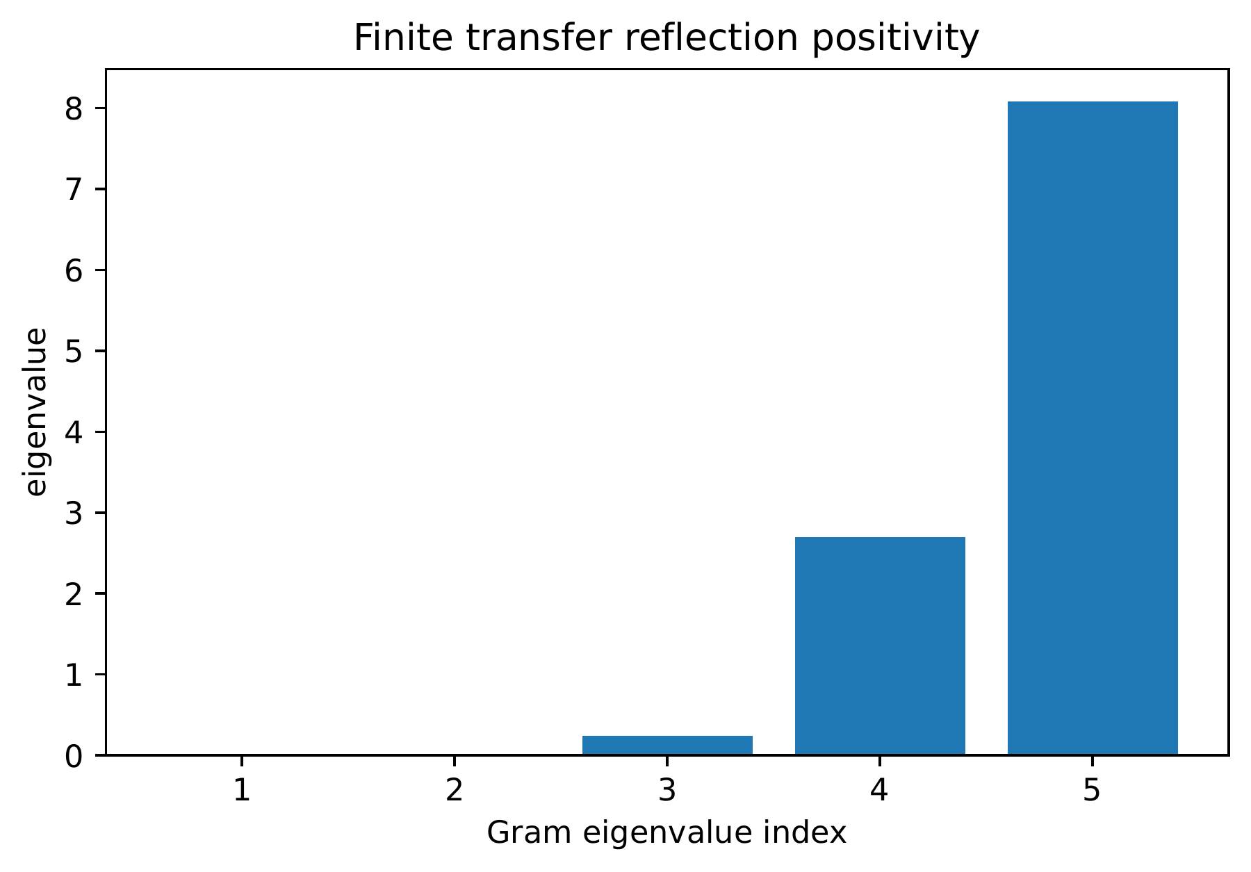
Text description
A bar chart lists five Gram-matrix eigenvalues with nonnegative displayed heights. The last eigenvalue is the largest. The manuscript separates a finite positivity check from the assumptions needed for a continuum transfer construction.
Proposition II.10.5: Ground packet convergence
Let \(P_0\) be the spectral projector of \(H\) at \(E_0\), and let
If an excited eigenvalue exists, then
Read proof · Visual guide: A positive transfer determines its Hamiltonian · Read statement and proof side by side · Permalink · Source line 1922 · Claim record · Lean coverage · Code · Worked examples
Proof of Proposition II.10.5
In the spectral decomposition, \(T^n-P_0\) has eigenvalues zero on the ground space and \({\mathrm e}^{-na(E_j-E_0)}\) on the excited eigenspaces. The largest is \({\mathrm e}^{-na\Delta}\).
Back to statement · Read statement and proof side by side · Permalink · Source line 1933 · Claim record · Lean coverage · Code · Worked examples
Proposition II.10.6: Symmetry resolved transfer
If \([H,P_a]=0\) for a complete packet family, then
and each reflection positive Gram matrix decomposes as the sum of its packet Gram matrices.
Read proof · Read statement and proof side by side · Permalink · Source line 1937 · Claim record · Lean coverage · Code · Worked examples
Proof of Proposition II.10.6
The functional calculus preserves commutation. Decompose every vector into packet components and use orthogonality.
Back to statement · Read statement and proof side by side · Permalink · Source line 1945 · Claim record · Lean coverage · Code · Worked examples
Finite reflection positivity is a necessary structural property of transfer data. It is not by itself the continuum Osterwalder Schrader theorem, which also requires a suitable algebra of Euclidean fields, covariance, regularity, clustering, and a controlled continuum limit [OsterwalderSchrader1973], [OsterwalderSchrader1975], [GlimmJaffe1987].
II.11 Finite spectral geometry and diffusion dimension
On this page · Permalink · Source line 1951
A finite spectral datum consists of a finite dimensional Hilbert space, a nonnegative self adjoint operator \(L\), and any declared packet family. One may take \(L=D^2\) for a finite Dirac type operator or a graph Laplacian. Related geometric viewpoints appear in [Connes1994], [Vassilevich2003].
Definition II.11.1: Heat trace and spectral dimension
Let the eigenvalues of \(L\) be \(\lambda_1,\ldots,\lambda_N\), with at least one zero eigenvalue. Define
and
Visual guide: A dimension curve is a scale diagnostic · Permalink · Source line 1955 · Claim record · Lean coverage · Code · Worked examples
Proposition II.11.2: Finite scale limits
For every finite nonnegative \(L\) with nontrivial kernel,
and
For every \(t>0\),
Read proof · Visual guide: A dimension curve is a scale diagnostic · Read statement and proof side by side · Permalink · Source line 1970 · Claim record · Lean coverage · Code · Worked examples
Proof of Proposition II.11.2
The formula in Definition II.11.1 is twice \(t\) times a weighted average of the eigenvalues. This gives the bound and the limit at zero. At large time, the denominator converges to \(\dim{\operatorname{Ker}} L\), while every positive eigenvalue contribution in the numerator decays exponentially.
Back to statement · Read statement and proof side by side · Permalink · Source line 1985 · Claim record · Lean coverage · Code · Worked examples
Thus a finite system cannot have a nonzero spectral dimension at the extreme ultraviolet or infrared ends. A geometric dimension can appear only in a refinement window.
Proposition II.11.3: Heat packet decomposition
If \([L,P_a]=0\) for every packet, then
The global spectral dimension is the average of the packet dimensions weighted by their heat traces:
where
for nonempty packet heat traces.
Read proof · Read statement and proof side by side · Permalink · Source line 1991 · Claim record · Lean coverage · Code · Worked examples
Proof of Proposition II.11.3
Commutation gives a block diagonal heat operator. Add the traces and the corresponding first spectral moments, then divide by the total heat trace.
Back to statement · Read statement and proof side by side · Permalink · Source line 2015 · Claim record · Lean coverage · Code · Worked examples
II.11.1 Periodic lattices
On this page · Permalink · Source line 2019
Let \(N\geq2\) and let \(\Lambda_N=({\mathbb Z}/N{\mathbb Z})^d\) be the unit flat torus grid with spacing \(1/N\). The standard periodic difference Laplacian has eigenvalues
where \(k\) runs through centered residue representatives. This is the standard periodic finite difference Laplacian [Strikwerda2004].
Theorem II.11.4: Low mode dispersion in dimension \(d\)
For every centered mode \(k\),
Read proof · Visual guide: Refine the grid while holding the mode fixed · Read statement and proof side by side · Permalink · Source line 2031 · Claim record · Lean coverage · Code · Worked examples
Proof of Theorem II.11.4
For \(x\in[0,\pi/2]\),
and
Thus
Apply this with \(x=\pi{\left\lvert k_j\right\rvert}/N\), multiply by \(4N^2\), and sum over \(j\).
Back to statement · Read statement and proof side by side · Permalink · Source line 2043 · Claim record · Lean coverage · Code · Worked examples
Theorem II.11.5: Fixed time heat trace convergence
For every \(t>0\),
as \(N\to\infty\). The first spectral moments also converge:
Consequently, the discrete spectral dimensions converge to the continuum torus spectral dimension at every fixed positive time.
Read proof · Visual guide: The dimension window has an order of limits · Read statement and proof side by side · Permalink · Source line 2059 · Claim record · Lean coverage · Code · Worked examples
Proof of Theorem II.11.5
For a fixed integer mode, Theorem II.11.4 gives
For centered modes, the inequality
gives
Also \(\lambda_N(k)\leq4\pi^2{\left\lvert k\right\rvert}^2\). Extend the discrete summands by zero outside the centered residue box. The heat trace terms are dominated by
and the moment terms by
Both dominating sequences are summable on \({\mathbb Z}^d\). Dominated convergence proves the two limits. Their quotient gives spectral dimension convergence.
Back to statement · Read statement and proof side by side · Permalink · Source line 2079 · Claim record · Lean coverage · Code · Worked examples
Standard fact II.11.6: Theta transformation
The continuum flat torus heat trace satisfies
This is the Poisson summation formula for a Gaussian.
Permalink · Source line 2105 · Claim record · Lean coverage · Code · Worked examples
Theorem II.11.7: Continuum torus small time dimension
Let
Then
as \(t\downarrow0\).
Read proof · Read statement and proof side by side · Permalink · Source line 2118 · Claim record · Lean coverage · Code · Worked examples
Proof of Theorem II.11.7
where
Differentiation gives
Substituting this estimate into the logarithmic derivative gives the stated small time expansion.
Back to statement · Read statement and proof side by side · Permalink · Source line 2133 · Claim record · Lean coverage · Code · Worked examples
Corollary II.11.8: Rigorous intermediate dimension window
For every \(\varepsilon>0\), there is a diffusion time \(t_\varepsilon>0\) and an integer \(N_\varepsilon\) such that
for every \(N\geq N_\varepsilon\).
Read proof · Visual guide: The dimension window has an order of limits · Read statement and proof side by side · Permalink · Source line 2151 · Claim record · Lean coverage · Code · Worked examples
Proof of Corollary II.11.8
Choose \(t_\varepsilon\) so that Theorem II.11.7 is within \(\varepsilon/2\) of \(d\). Then apply Theorem II.11.5 to choose \(N_\varepsilon\) so that the discrete spectral dimension is within \(\varepsilon/2\) of the continuum value.
Back to statement · Read statement and proof side by side · Permalink · Source line 2159 · Claim record · Lean coverage · Code · Worked examples
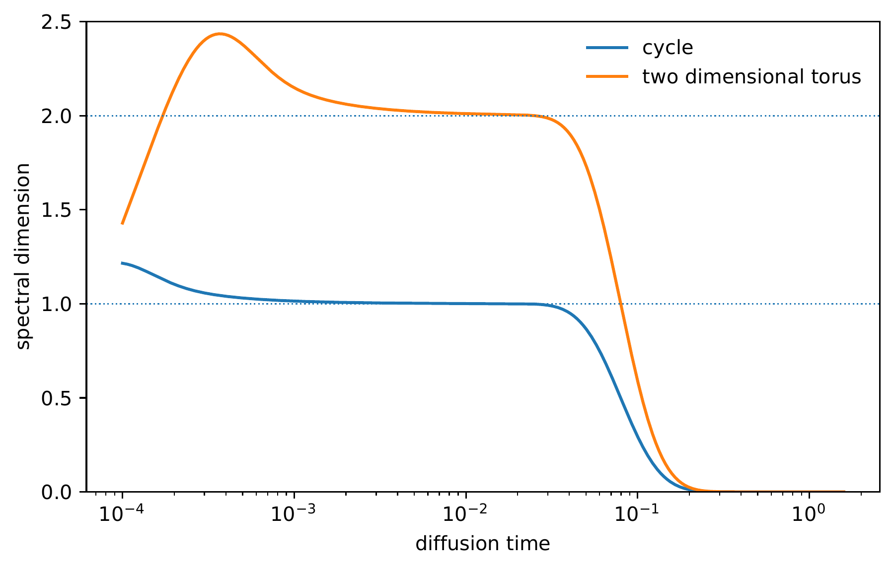
Text description
The cycle curve approaches a window near one and the two-dimensional torus curve a window near two. Both ultimately decay toward zero at long diffusion times. These finite-window diagnostics are not proofs of a physical continuum dimension.
The order of limits matters. Taking \(t\downarrow0\) at fixed \(N\) gives zero. Taking \(N\to\infty\) at fixed positive \(t\), then taking \(t\downarrow0\), gives the continuum dimension.
II.12 Constraint closure and anomaly packets
On this page · Permalink · Source line 2172
Let \(C_1,\ldots,C_m\) be self adjoint constraint operators on a finite dimensional Hilbert space. The distinction between constraint action and constraint closure is standard in constrained Hamiltonian theory [Dirac1964], [HenneauxTeitelboim1992]. Write
Definition II.12.1: Universal closure obstruction
Let
be the quotient map. Define
Permalink · Source line 2180 · Claim record · Lean coverage · Code · Worked examples
Theorem II.12.2: Finite constraint closure criterion
The constraint span \(\mathfrak c\) is closed under commutators exactly when
for all \(a,b\).
Read proof · Visual guide: A zero compressed anomaly can be automatic · Visual guide: Transport constraints without hiding closure · Read statement and proof side by side · Permalink · Source line 2193 · Claim record · Lean coverage · Code · Worked examples
Proof of Theorem II.12.2
The quotient class vanishes exactly when \([C_a,C_b]\in\mathfrak c\). This holds for every pair exactly when \(\mathfrak c\) is a Lie algebra under the commutator.
Back to statement · Read statement and proof side by side · Permalink · Source line 2201 · Claim record · Lean coverage · Code · Worked examples
If structure coefficients \(f_{ab}^{\phantom{ab}c}\) are prescribed, define the fixed structure anomaly
Exact realization of the prescribed algebra is the stronger condition \(\mathfrak A_{ab}=0\).
Proposition II.12.3: Physical compression is not a closure test
Let
and let \(P_{{\mathrm{phys}}}\) be its orthogonal projector. Then
for every pair \(a,b\), whether or not the constraint span closes.
Read proof · Visual guide: A zero compressed anomaly can be automatic · Read statement and proof side by side · Permalink · Source line 2214 · Claim record · Lean coverage · Code · Worked examples
Proof of Proposition II.12.3
Self adjointness and \(C_aP_{{\mathrm{phys}}}=0\) give \(P_{{\mathrm{phys}}}C_a=0\). Both terms in the compressed commutator therefore vanish.
Back to statement · Read statement and proof side by side · Permalink · Source line 2226 · Claim record · Lean coverage · Code · Worked examples
The quotient in Definition II.12.1 is needed because closure concerns the operator algebra. Compression to physical states tests only the action on the common kernel, where the constraints already vanish.
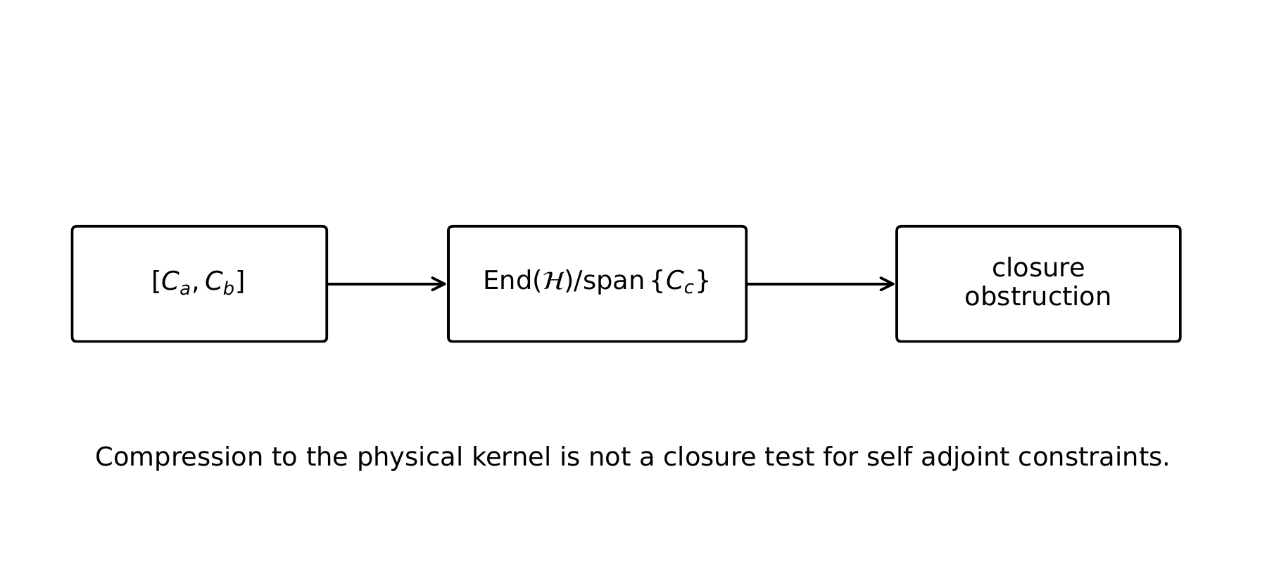
Text description
Three boxes connect a constraint commutator to the operator-space quotient by the constraint span and then to the closure obstruction. The accompanying note says that compression to the physical kernel cannot replace this closure test for self-adjoint constraints.
Theorem II.12.4: Invariance of the physical space
Let \(H=H^*\). Suppose
for every \(a\). Then \(H\) preserves \({\mathcal H}_{{\mathrm{phys}}}\), and so does \({\mathrm e}^{-{\mathrm i} tH}\) for every real \(t\).
Read proof · Read statement and proof side by side · Permalink · Source line 2239 · Claim record · Lean coverage · Code · Worked examples
Proof of Theorem II.12.4
For \(\psi\in{\mathcal H}_{{\mathrm{phys}}}\),
Thus \(H\psi\in{\mathcal H}_{{\mathrm{phys}}}\). The exponential preserves every invariant finite dimensional subspace.
Back to statement · Read statement and proof side by side · Permalink · Source line 2249 · Claim record · Lean coverage · Code · Worked examples
II.12.1 Constraint refinement
On this page · Permalink · Source line 2259
Let \(({\mathcal H}_\ell,C_{\ell,a})\) and \(({\mathcal H}_{\ell+1},C_{\ell+1,a})\) be two levels, and let
be an isometry.
Theorem II.12.5: Exact constraint transport
Assume
for every \(a\). Then
If the same structure coefficients are used at both levels, then
The isometry maps coarse physical states into fine physical states.
Read proof · Visual guide: Transport constraints without hiding closure · Read statement and proof side by side · Permalink · Source line 2267 · Claim record · Lean coverage · Code · Worked examples
Proof of Theorem II.12.5
Apply the intertwining identity twice to each product in the commutator. The anomaly identity follows by subtracting the same linear combination of constraints. If \(C_{\ell,a}\psi=0\), then
Back to statement · Read statement and proof side by side · Permalink · Source line 2287 · Claim record · Lean coverage · Code · Worked examples
Proposition II.12.6: Approximate constraint transport
Assume
and
Then a coarse physical unit vector \(\psi\) satisfies
Also,
Read proof · Visual guide: Transport constraints without hiding closure · Read statement and proof side by side · Permalink · Source line 2294 · Claim record · Lean coverage · Code · Worked examples
Proof of Proposition II.12.6
The first claim follows by applying the intertwining defect to \(\psi\). Write
Expanding the two commutators gives four error terms:
The triangle inequality and the stated bounds on the constraints and defects give the claimed estimate.
Back to statement · Read statement and proof side by side · Permalink · Source line 2321 · Claim record · Lean coverage · Code · Worked examples
Approximate transport controls finite violations. It does not turn a nonzero anomaly into an exact continuum algebra without a limit theorem and a common operator domain.
II.13 Quantum refinement towers
On this page · Permalink · Source line 2341
Definition II.13.1: Finite quantum refinement tower
A finite quantum refinement tower consists of Hilbert spaces \({\mathcal H}_\ell\), isometries
self adjoint Hamiltonians \(H_\ell\), packet projectors \(P_{\ell,a}\), constraints \(C_{\ell,r}\), and positive transfer operators \(T_\ell\). Exact compatibility means that every declared object intertwines with \(R_\ell\). Approximate compatibility is recorded by the corresponding operator norm defects.
Permalink · Source line 2343 · Claim record · Lean coverage · Code · Worked examples
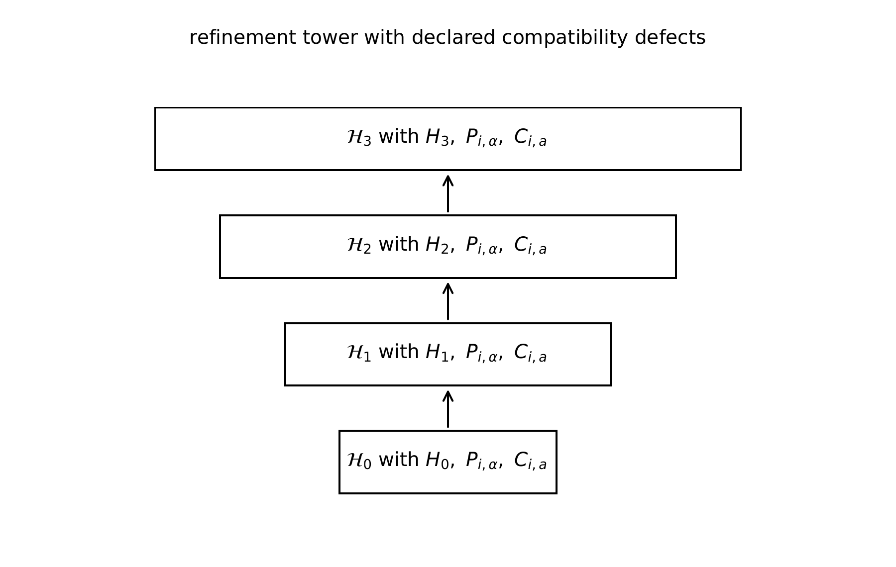
Text description
Four vertically stacked Hilbert-space levels are connected by refinement arrows. Each level lists its Hamiltonian, packet family, and constraints. The tower keeps the corresponding compatibility defects as separate requirements.
II.13.1 Exact bounded direct limits
On this page · Permalink · Source line 2358
Let \({\mathcal H}_\infty\) be the Hilbert direct limit of the isometric system, and let
be the canonical isometries.
Theorem II.13.2: Bounded Hamiltonian direct limit
Assume
and
Then there is a unique bounded self adjoint operator \(H_\infty\) on \({\mathcal H}_\infty\) such that
for every \(\ell\). It satisfies
and
when the Hamiltonians are nonnegative.
Read proof · Visual guide: Two routes to a bounded Hamiltonian limit · Read statement and proof side by side · Permalink · Source line 2366 · Claim record · Lean coverage · Code · Worked examples
Proof of Theorem II.13.2
Define \(H_\infty\) on the algebraic union of the embedded levels by
Compatibility makes the definition independent of the chosen level. The uniform norm bound makes the operator bounded on the dense union, so it extends uniquely to the completion. It is symmetric because every \(H_\ell\) is self adjoint. A bounded symmetric operator defined on the whole Hilbert space is self adjoint. The functional calculus intertwining follows first for polynomials and then for exponentials by uniform convergence.
Back to statement · Read statement and proof side by side · Permalink · Source line 2394 · Claim record · Lean coverage · Code · Worked examples
Theorem II.13.3: Exact packet direct limit
Assume the packet families have one fixed finite address set at every level and each packet address \(a\) is compatible in the sense
Then there is an orthogonal projector \(P_{\infty,a}\) on \({\mathcal H}_\infty\) satisfying
Finite completeness and orthogonality pass to the direct limit.
Read proof · Read statement and proof side by side · Permalink · Source line 2402 · Claim record · Lean coverage · Code · Worked examples
Proof of Theorem II.13.3
Use the same construction as in Theorem II.13.2. Every projector has norm at most one, so no additional boundedness assumption is needed. The projector identities hold on the dense algebraic union and hence on the completion.
Back to statement · Read statement and proof side by side · Permalink · Source line 2414 · Claim record · Lean coverage · Code · Worked examples
II.13.2 Norm summable approximation
On this page · Permalink · Source line 2418
The next theorem places all approximating Hamiltonians on a common Hilbert space. It applies to bounded effective Hamiltonians. An unbounded field Hamiltonian requires a different convergence argument.
Theorem II.13.4: Norm summable Hamiltonian tower
Let \((H_n)\) be bounded self adjoint operators on one Hilbert space and assume
Then \(H_n\) converges in norm to a bounded self adjoint operator \(H\). For every \(T>0\),
If every \(H_n\geq0\), then
Read proof · Visual guide: Two routes to a bounded Hamiltonian limit · Read statement and proof side by side · Permalink · Source line 2422 · Claim record · Lean coverage · Code · Worked examples
Proof of Theorem II.13.4
The summability condition makes \((H_n)\) Cauchy in operator norm. The limit is self adjoint. Duhamel's identity gives
Both unitary factors have norm one, which gives the first estimate. The same argument gives the Euclidean estimate because the semigroups generated by nonnegative Hamiltonians are contractions.
Back to statement · Read statement and proof side by side · Permalink · Source line 2443 · Claim record · Lean coverage · Code · Worked examples
Corollary II.13.5: Limit of packet leakage
Let \(P_n\) be orthogonal projectors and \(H_n\) bounded self adjoint operators on one Hilbert space, with \(P_n\to P\) and \(H_n\to H\) in norm. Then for every bounded time interval,
uniformly in time.
Read proof · Visual guide: Two routes to a bounded Hamiltonian limit · Read statement and proof side by side · Permalink · Source line 2453 · Claim record · Lean coverage · Code · Worked examples
Proof of Corollary II.13.5
Add and subtract terms so that one factor changes at a time. The projector terms converge uniformly because \(P_n\to P\) in norm. Duhamel's identity gives
which proves uniform convergence of the middle factor.
Back to statement · Read statement and proof side by side · Permalink · Source line 2463 · Claim record · Lean coverage · Code · Worked examples
Theorem II.13.6: Reflection positivity is closed under limits
Suppose \(C_n(j,k)\) are reflection positive kernels on \({\mathbb N}\), meaning every finite matrix
is positive semidefinite. If
for every pair, then \(C\) is reflection positive.
Read proof · Visual guide: Choose the topology that preserves the quantity · Read statement and proof side by side · Permalink · Source line 2474 · Claim record · Lean coverage · Code · Worked examples
Proof of Theorem II.13.6
For a fixed finite set of times and coefficients, the corresponding quadratic forms are nonnegative and converge to the quadratic form of \(C\). The limit is nonnegative.
Back to statement · Read statement and proof side by side · Permalink · Source line 2486 · Claim record · Lean coverage · Code · Worked examples
Theorem II.13.7: Constraint closure under norm convergence
Let \(C_{n,a}\to C_a\) in norm for every \(a\), and fix structure coefficients \(f_{ab}^{\phantom{ab}c}\). If
then
Read proof · Read statement and proof side by side · Permalink · Source line 2490 · Claim record · Lean coverage · Code · Worked examples
Proof of Theorem II.13.7
Operator multiplication and the commutator are continuous in operator norm. Pass to the limit in the anomaly identity.
Back to statement · Read statement and proof side by side · Permalink · Source line 2506 · Claim record · Lean coverage · Code · Worked examples
Theorem II.13.8: Heat trace convergence from trace norm
Let \(L_n,L\) be nonnegative self adjoint operators on one Hilbert space. For a fixed \(t>0\), assume their heat operators are trace class and that
in trace norm. Then
If also the heat moment operators are trace class and
in trace norm and the limiting heat trace is nonzero, then the spectral dimensions defined by the heat moment ratio converge at that time.
Read proof · Visual guide: Choose the topology that preserves the quantity · Read statement and proof side by side · Permalink · Source line 2510 · Claim record · Lean coverage · Code · Worked examples
Proof of Theorem II.13.8
The trace is continuous in trace norm. Apply this to the heat operators and to the first heat moments, then take the quotient in Definition II.11.1.
Back to statement · Read statement and proof side by side · Permalink · Source line 2526 · Claim record · Lean coverage · Code · Worked examples
Remark II.13.9
The theorems above produce bounded continuum Hamiltonians. A physically useful continuum Hamiltonian is often unbounded. Its construction generally requires strong resolvent convergence, convergence of closed quadratic forms, or another method that controls operator domains [Kato1995], [ReedSimon1972]. None of those conclusions follows from finite matrix convergence without additional hypotheses.
II.14 Continuum milestones and exact boundary
On this page · Visual guide: What these pictures establish · Visual guide: Choose the topology that preserves the quantity · Permalink · Source line 2534
The finite theorems establish exact identities and criteria for bounded limits. Passing from a finite transfer model to a continuum theory still requires several separate arguments. This section states those remaining mathematical tasks.
Definition II.14.1: Anomaly free continuum constraint system
A continuum constraint system consists of a Hilbert space, a common invariant dense domain \({\mathcal D}\), and operators \(C_a\) on \({\mathcal D}\). It is anomaly free for prescribed structure coefficients when
for every \(\psi\in{\mathcal D}\), and when the associated gauge evolution is defined on the physical quotient or physical subspace.
Permalink · Source line 2538 · Claim record · Lean coverage · Code · Worked examples
Norm closure of bounded finite constraints, as in Theorem II.13.7, is one special case. It does not treat unbounded constraints, changing domains, structure functions, or renormalized operator products.
Definition II.14.2: Reflection positive Euclidean limit
A reflection positive Euclidean limit requires a limiting algebra of observables, Euclidean time translations, a reflection operation, and correlation functions whose reflected quadratic forms are nonnegative. A field theoretic reconstruction also requires the regularity and covariance assumptions needed to construct a Hilbert space, a vacuum, and a self adjoint time translation generator.
Permalink · Source line 2550 · Claim record · Lean coverage · Code · Worked examples
Theorem II.13.6 shows that positivity of each fixed finite Gram matrix survives pointwise convergence. It does not prove existence, locality, clustering, or the remaining Osterwalder Schrader axioms.
Definition II.14.3: Einstein infrared criterion
A quantum geometric tower meets an Einstein infrared criterion only if an effective action is controlled at long wavelengths and has an expansion whose leading geometric terms take the form
Here the volume coefficient includes the sign and normalization written explicitly in the cosmological term in Part I. The expansion must respect the limiting gauge identities and must include an estimate for the omitted terms on the declared infrared regime.
Permalink · Source line 2556 · Claim record · Lean coverage · Code · Worked examples
A spectral dimension close to four does not imply this criterion. A heat trace records eigenvalue growth. It does not determine the tensor structure, gauge identities, sign, or interaction coefficients of an effective action.
Definition II.14.4: Massless spin two criterion
A positive massless spin two sector requires a physical two point function or resolvent with a massless pole in the transverse traceless sector, positive residue on physical states, absence of negative norm modes, and compatibility with the limiting gauge constraints. Interactions must preserve the constraint structure.
Permalink · Source line 2577 · Claim record · Lean coverage · Code · Worked examples
A low energy eigenvalue, a spectral dimension plateau, or a finite rank two tensor packet does not establish a massless spin two particle.
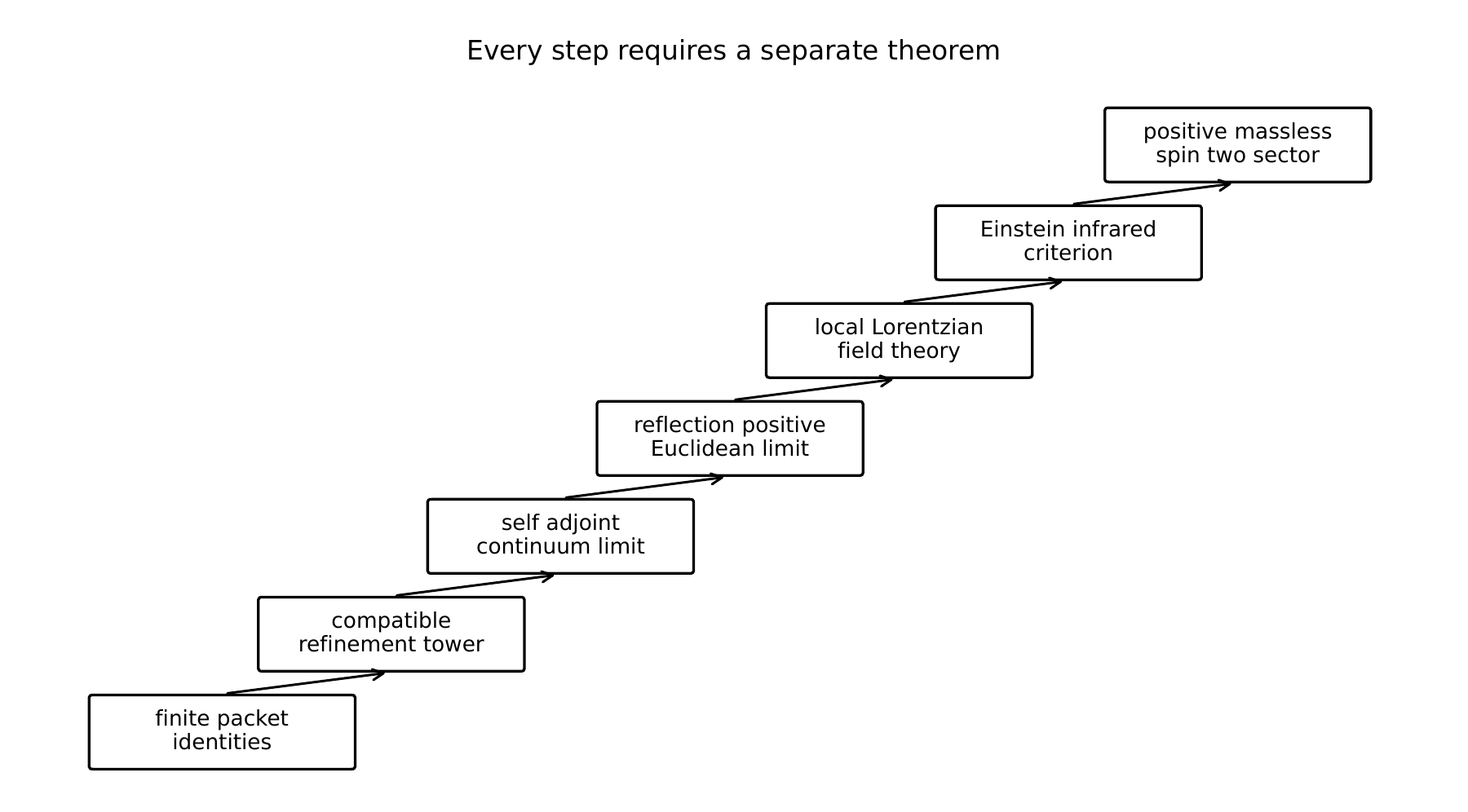
Text description
Seven steps progress from finite packet identities through compatible refinement, a self-adjoint continuum limit, a reflection-positive Euclidean limit, local Lorentzian field theory, an Einstein infrared criterion, and a positive massless spin-two sector. Each later step requires its own theorem; the diagram does not assert that the chain has been completed.
| Milestone | Finite result available here | Missing continuum input |
|---|---|---|
| Symmetry and constraints | exact packets and quotient obstruction | common unbounded domain and renormalized closure |
| Effective dynamics | exact Feshbach map and uniform gap bounds | cutoff independent spectral separation and locality |
| Euclidean transfer | positive finite transfer and finite reflection positivity | convergent Euclidean fields and reconstruction axioms |
| Spectral dimension | lattice heat trace convergence | relation to a physical metric and interacting observables |
| Lorentzian theory | bounded unitary direct limits | unbounded generator, causality, locality, and field algebra |
| Einstein regime | a definition of the required expansion | derivation and error control for the effective action |
| Spin two sector | a precise spectral criterion | positive physical pole and interaction consistency |
II.15 Conclusion
On this page · Permalink · Source line 2610
A complete packet family gives one coordinate language for finite quantum structure. Group characters produce symmetry packets. Charged operators obey exact selection rules. Circuits become coherent sums over packet paths. The canonical moving connection separates geometric transport from physical mixing. Density matrices and channels use two sided packets, while channel covariance becomes block preservation on operator space and symmetry of the Choi matrix.
Compression to a code gives a natural error correction obstruction. Its vanishing is the Knill Laflamme condition. Diagonalizing the resulting coefficient matrix produces orthogonal syndrome packets and an exact recovery on the error span. Schur Feshbach elimination gives an equally exact description of hidden Hamiltonian packets. Their frequency response is the self energy, and their time response is a positive definite memory kernel.
Positive Euclidean transfer gives finite reflection positivity. Periodic lattice heat traces converge to the continuum torus at every fixed positive diffusion time, and the continuum small time spectral dimension is recovered after the refinement limit. Constraint closure is measured by a quotient of operator space, not by compression to the physical kernel.
The theorems for bounded towers show how exact compatibility and summable differences in operator norm produce limiting quantum evolutions. Their hypotheses also mark the scope of the argument. Unbounded field Hamiltonians, continuum gauge constraints, reflection positive field measures, the Einstein infrared action, and a massless spin two sector each require additional theorems. The finite packet calculus gives a common framework in which those questions can be stated and studied, while leaving their physical resolution open.