
For a two-level system, choose \(H=\varepsilon X\), \(P={\left|0\right\rangle}{\left\langle0\right|}\), and \(Q=I-P\). Direct exponentiation gives
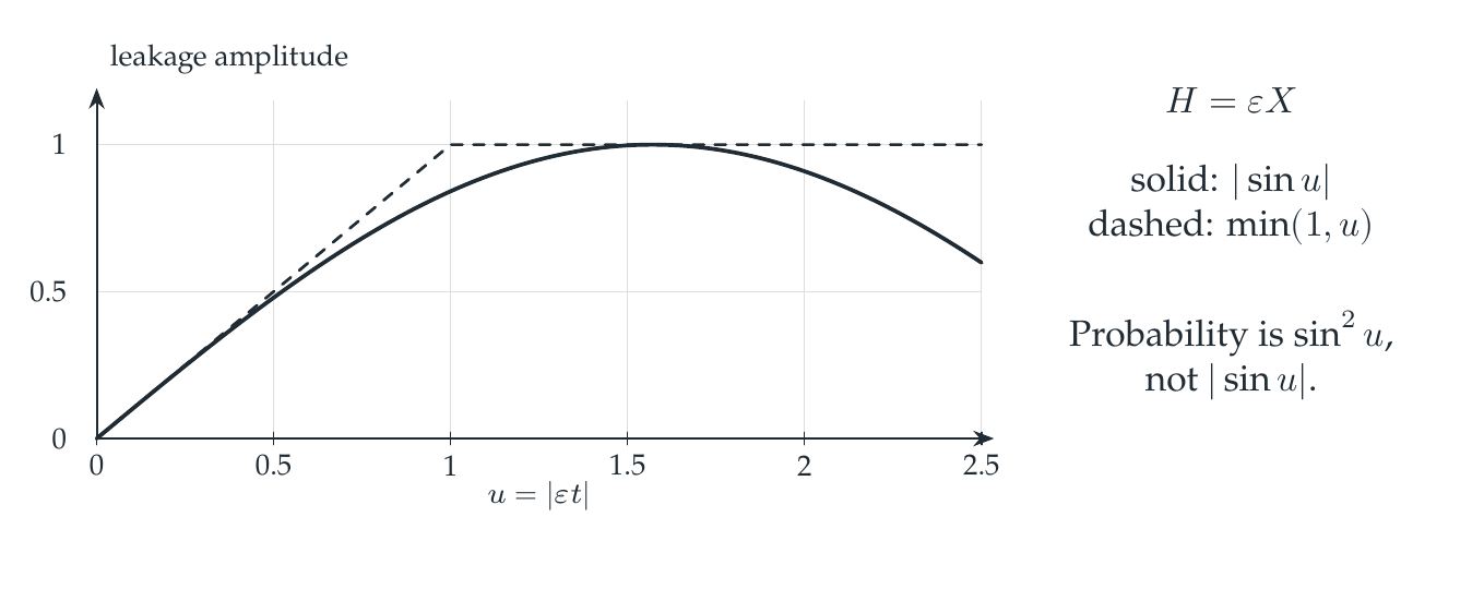
The general commutator estimate becomes the elementary bound \(|\sin u|\le |u|\). Unitarity also bounds the amplitude by one.
Reading the drawing
The horizontal axis is scaled elapsed time. The solid curve is the absolute sine amplitude and the dashed curve is the stated upper bound. The note on the right distinguishes this amplitude from the squared transition probability.
Drawing labels and data 14 labels
Read the original labels as selectable text. Tables preserve grid relationships; other short labels are grouped compactly.
- 0
- 0.5
- 1
- 1.5
- 2
- 2.5
- 0
- 0.5
- 1
- \(u=|\varepsilon t|\)
- leakage amplitude
- \(H=\varepsilon X\)
solid: \(|\sin u|\)
dashed: \(\min(1,u)\)
Probability is \(\sin^2u\),
not \(|\sin u|\).
From a norm to a probability
For this initial state, the escape probability is \(\sin^2(\varepsilon t)\), not \(|\sin(\varepsilon t)|\). Consequently
At \(\varepsilon t=\pi/6\), the amplitude is \(1/2\) and the probability is \(1/4\). Near zero, amplitudes are first order while escape probabilities are second order. Mixing those two quantities produces an incorrect interpretation of a leakage plot.
The figure displays samples of the explicit functions above. The supporting check verifies the exact exponential identity, its unitarity, the squared leakage matrix, and the special-time value. The paper's theorem supplies the bound for all times within its stated scope.
At larger times amplitude can return from the hidden packet. The commutator bound therefore limits the largest possible leakage without predicting that it must rise monotonically.
Read this as
The norm estimate controls amplitude. For a normalized state, square it to obtain a probability bound, and retain the distinction between a bound and the actual oscillatory dynamics.