
Set the laboratory Hamiltonian to zero and keep \(\psi(t)={\left|0\right\rangle}\) fixed. Describe it in rotating coordinates,
The vector has not moved in the laboratory, but its coordinate entries have changed.
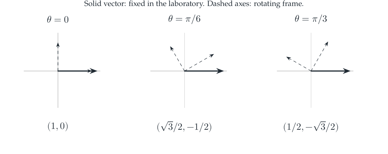
Reading the drawing
The solid arrow stays fixed while the dashed coordinate axes rotate from left to right. The coordinate pairs below the panels change even though the laboratory vector does not.
Drawing labels and data 7 labels
Read the original labels as selectable text. Tables preserve grid relationships; other short labels are grouped compactly.
- \(\theta=0\)
- \((1,0)\)
- \(\theta=\pi/6\)
- \((\sqrt3/2,-1/2)\)
- \(\theta=\pi/3\)
- \((1/2,-\sqrt3/2)\)
Solid vector: fixed in the laboratory. Dashed axes: rotating frame.
The missing term can be computed exactly
Let \(J={\begin{pmatrix}0&-1\\1&0\end{pmatrix}}\). Since \(U^*\dot U=J\), the coordinate Hamiltonian is
This matrix is Hermitian. Omitting it would predict a constant \(y\), contradicting the displayed coordinates. In this example the norm of the omitted time derivative is exactly one, so the failure is not a small numerical residual.
For a nonzero laboratory Hamiltonian, the same product rule adds the transformed physical term \(U^*HU\). Thus \(U^*HU-{\mathrm i} U^*\dot U\) separates the physical generator from the coordinate correction. Both pieces belong to the same equation but have different origins.
The drawing shows actual rotated axes at three angles, not three different laboratory trajectories. The check differentiates the exact matrices and verifies the coordinate Schrödinger equation symbolically. The explicit derivatives make a numerical difference approximation unnecessary.
Read this as
When coordinates move, even a stationary physical vector acquires changing components. The connection term accounts for that change without adding a force to the laboratory system.