
For the unit circle grid with \(N\) sites, the scaled eigenvalues are \(\lambda_N(k)=4N^2\sin^2(\pi k/N)\). Put \(Z_N(t)=\sum_ke^{-t\lambda_N(k)}\) and \(d_N(t)=2t\sum_k\lambda_N(k)e^{-t\lambda_N(k)}/Z_N(t)\).
At the single time \(t=\log2/16\), two small grids admit exact rational heat weights:
These are unnormalized traces. Normalizing by \(N\) changes \(Z_N\) but leaves the logarithmic derivative at that fixed grid unchanged.
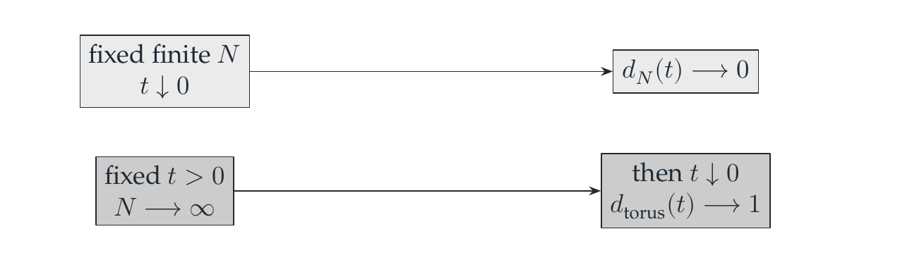
Reading the drawing
The top route keeps a finite grid fixed while time goes to zero. The bottom route first refines the grid at fixed positive time and then takes the small-time limit. The arrows retain the distinct outcomes stated in the source.
Drawing labels and data 4 labels
Read the original labels as selectable text. Tables preserve grid relationships; other short labels are grouped compactly.
fixed finite \(N\)
\(t\downarrow0\)
- \(d_N(t)\longrightarrow0\)
fixed \(t>0\)
\(N\longrightarrow\infty\)
then \(t\downarrow0\)
\(d_{\rm torus}(t)\longrightarrow1\)
The theorem uses two separate choices
For each \(\varepsilon>0\), first choose a fixed positive time \(t_\varepsilon\) so that the continuum torus dimension differs from one by less than \(\varepsilon/2\). Then choose \(N_\varepsilon\) so that every \(N\geq N_\varepsilon\) differs from that continuum value by less than \(\varepsilon/2\) at the same time. This proves one controlled intermediate time for all sufficiently fine grids.
It does not assert a uniform interval width from that argument, a moving time \(t_N\) with no extra estimates, or a dimension plateau at every scale. At fixed finite \(N\), \(d_N(t)\to0\) as \(t\downarrow0\) and as \(t\to\infty\). By contrast, first taking \(N\to\infty\) at positive \(t\) and then taking \(t\downarrow0\) yields the continuum dimension.
Where the infinite tail is controlled
At a fixed time, the proof bounds centered modes below by \(16k^2\) and above by \(4\pi^2k^2\). The summable Gaussian dominators control both the heat trace and its first moment. A finite grid table supplies neither those tails nor the quantifiers. The retained check verifies the two displayed spectra, rational weights, traces, and dimension coefficients. It also distinguishes the unscaled cycle with four sites from the scaled unit circle grid.
Read this as
The strengthened window result proves convergence after fixing a suitable time. The exact table is a worked calculation, not its proof.