
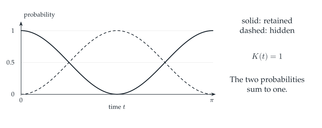
Choose \(H=X\), initial state \((1,0)^T\), and retain the first coordinate. The coupled equations and their solution are
The hidden probability returns periodically. Deleting the hidden row and column would instead leave the zero Hamiltonian and predict \(x(t)=1\).
Reading the drawing
The solid retained curve and dashed hidden curve start at opposite endpoints, exchange, and return. Their sum and the memory-kernel value are annotated on the right. The horizontal axis is real time.
Drawing labels and data 10 labels
Read the original labels as selectable text. Tables preserve grid relationships; other short labels are grouped compactly.
- 0
- 0
- 0.5
- 1
- time \(t\)
- probability
solid: retained
dashed: hidden
- \(K(t)=1\)
The two probabilities
sum to one.
- \(\pi\)
Eliminate exactly, not approximately
Integrating the second equation with \(y(0)=0\) gives \(y(t)=-{\mathrm i}\int_0^tx(s)\,ds\). Substitution produces
The memory kernel is the constant function one. Differentiating once more recovers \(\ddot x=-x\) with \(x(0)=1\) and \(\dot x(0)=0\), explaining the cosine solution. A nonzero hidden initial state would add a forcing term that must also be retained.
The full propagator is a unitary group, but its retained scalar entry is not a semigroup. At \(t=s=\pi/4\),
There is no contradiction: compression of a product need not equal the product of the compressed factors when the hidden subspace carries intermediate amplitude.
The check verifies the differential and integral equations symbolically and the displayed nonzero semigroup defect exactly. The curves visualize the explicit solution and its periodic return of amplitude.
Read this as
Exact elimination replaces a hidden coordinate with memory and forcing from the initial data. Replacing that memory by a constant generator is an additional approximation, not part of the exact theorem.