
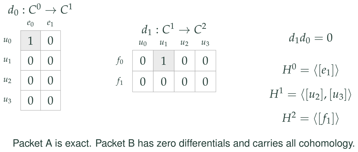
Over \({\mathbb F}_5\), use bases \((e_0,e_1)\), \((u_0,u_1,u_2,u_3)\), and \((f_0,f_1)\) in degrees zero, one, and two. The only nonzero differential values are \(d_0e_0=u_0\) and \(d_1u_1=f_0\). Consequently \(d_1d_0=0\).
Reading the drawing
Two differential matrices map the displayed coordinate bases across degrees zero, one and two. One packet is exact; the other has zero differential and carries the surviving classes. The surviving cohomology classes are listed at the right.
Drawing labels and data 35 labels
Read the original labels as selectable text. Tables preserve grid relationships; other short labels are grouped compactly.
- \(d_0:C^0\to C^1\)
| Row / column | \(e_0\) | \(e_1\) |
|---|---|---|
| \(u_0\) | \(1\) | \(0\) |
| \(u_1\) | \(0\) | \(0\) |
| \(u_2\) | \(0\) | \(0\) |
| \(u_3\) | \(0\) | \(0\) |
- \(d_1:C^1\to C^2\)
| Row / column | \(u_0\) | \(u_1\) | \(u_2\) | \(u_3\) |
|---|---|---|---|---|
| \(f_0\) | \(0\) | \(1\) | \(0\) | \(0\) |
| \(f_1\) | \(0\) | \(0\) | \(0\) | \(0\) |
- \(d_1d_0=0\)
- \(H^0=\langle[e_1]\rangle\)
- \(H^1=\langle[u_2],[u_3]\rangle\)
- \(H^2=\langle[f_1]\rangle\)
Packet A is exact. Packet B has zero differentials and carries all cohomology.
The quotient is the important step
In degree one, the cycles are \({\operatorname{span}}(u_0,u_2,u_3)\), but \(u_0\) is a boundary. Thus the cohomology is represented by \(u_2,u_3\), not by every vector killed by \(d_1\). In the other degrees the surviving classes are \(e_1\) and \(f_1\).
Packet A contains \(e_0\), \(u_0,u_1\), and \(f_0\). It is exact and contributes \((0,0,0)\). Packet B contains \(e_1\), \(u_2,u_3\), and \(f_1\), with zero differentials, and contributes \((1,2,1)\). Adding the packet cohomologies reconstructs the total.
The projectors must be specified in every degree and commute with the differential. Their existence is not a consequence of the printed dimensions. Identifying this finite complex with the actual continuous cohomology of an arithmetic deformation problem would also require a separate comparison.
Read this as
Resolve the differential first, then pass from cycles to classes. Counting packet dimensions alone does not compute cohomology.