
Return to the two operators from Visual 9. The exact product representation has diagonal part \(D_AD_B\) and two-column correction factors \(U_C,V_C\). Apply it to the original \(x=(1,-1,2,0,-2,3)^T\).
Reading the drawing
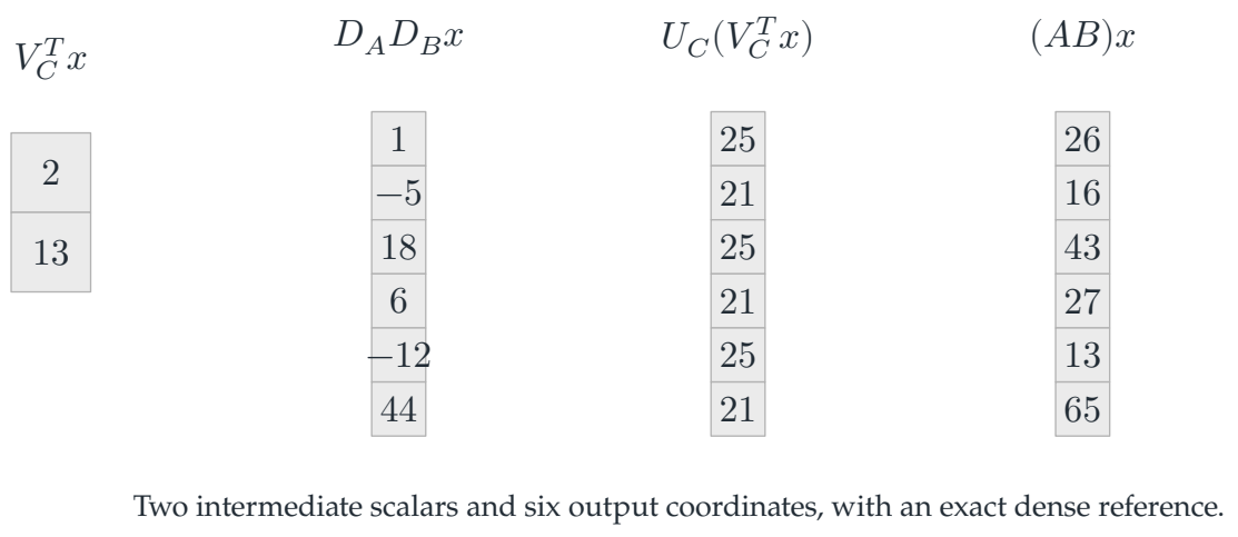
The displayed calculation follows the running input through the local product and low-rank correction. Their sum is compared with an independent dense reference.
Drawing labels and data 25 labels
Read the original labels as selectable text. Tables preserve grid relationships; other short labels are grouped compactly.
- \(V_C^Tx\)
- \(2\)
- \(13\)
- \(D_AD_Bx\)
- \(1\)
- \(-5\)
- \(18\)
- \(6\)
- \(-12\)
- \(44\)
- \(U_C(V_C^Tx)\)
- \(25\)
- \(21\)
- \(25\)
- \(21\)
- \(25\)
- \(21\)
- \((AB)x\)
- \(26\)
- \(16\)
- \(43\)
- \(27\)
- \(13\)
- \(65\)
Two intermediate scalars and six output coordinates, with an exact dense reference.
A complete reader calculation
The local contribution is \((1,-5,18,6,-12,44)^T\). The correction is \((25,21,25,21,25,21)^T\). Their sum is
The checker forms the dense matrices \(A\) and \(B\) independently, multiplies them, applies the product to \(x\), and compares all six components. The dense array is a validation reference, not a requirement of the factored application route.
Choose what happens next
For another input, reuse the factors. For a required explicit matrix, pay materialization. For a long product chain, track rank growth and decide whether recompression is useful. If approximation is introduced, transport its error through the later operators rather than reporting only a local singular tail.
This small example does not predict a speedup: at dimension six, implementation overhead can dominate. Its purpose is to make the semantics auditable. The same identity can then be used inside a larger, separately benchmarked workload.
Read this as
The full route is: represent the exact operator, retain every interaction, return the requested object, and validate against an independent reference. Performance is a further experiment.