
A dense array, a factored operator, and a compiled execution plan are different objects. They may denote the same linear map, but they need not store the same data, return the same output, or incur the same costs. This guide makes those distinctions visible through calculations rather than a pipeline of boxes.
Reading the drawing
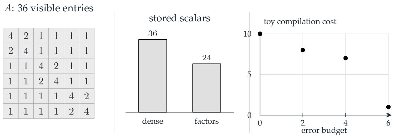
The panels show a dense array, storage counts for dense and factored forms, and toy compilation costs under different error budgets. The cost plot uses declared model values rather than measured timings.
Drawing labels and data 51 labels
Read the original labels as selectable text. Tables preserve grid relationships; other short labels are grouped compactly.
- \(A\): 36 visible entries
| Row / column | Column 1 | Column 2 | Column 3 | Column 4 | Column 5 | Column 6 |
|---|---|---|---|---|---|---|
| Row 1 | \(4\) | \(2\) | \(1\) | \(1\) | \(1\) | \(1\) |
| Row 2 | \(2\) | \(4\) | \(1\) | \(1\) | \(1\) | \(1\) |
| Row 3 | \(1\) | \(1\) | \(4\) | \(2\) | \(1\) | \(1\) |
| Row 4 | \(1\) | \(1\) | \(2\) | \(4\) | \(1\) | \(1\) |
| Row 5 | \(1\) | \(1\) | \(1\) | \(1\) | \(4\) | \(2\) |
| Row 6 | \(1\) | \(1\) | \(1\) | \(1\) | \(2\) | \(4\) |
- stored scalars
- dense
- \(36\)
- factors
- \(24\)
- 0
- 2
- 4
- 6
- 0
- 5
- 10
- error budget
- toy compilation cost
Three models to carry through the paper
The first is a six-dimensional operator \(A=D+uv^T\). Every entry of \(A\) is nonzero, yet three \(2\times2\) diagonal blocks and two thin vectors suffice to apply it exactly. Pages Visual 3, Visual 9, Visual 10, and Visual 27 reuse this operator or its factors.
The second starts with redundant factors \(L\) and \(R\). Actual range coordinates reduce a \(4\times3\) product to a \(2\times3\) core. Pages Visual 11–Visual 12 connect rank, singular tails, and the geometric reason a small-core optimum is also an ambient optimum.
The third is a seven-node candidate tree with exactly five prunings. Its budget optimum is not selected by any Lagrangian penalty. Pages Visual 21–Visual 23 let readers inspect every feasible choice and every changed subproblem.
How to use the guide
A source line beneath each title identifies the relevant final traditional result; the accompanying source crosswalk records its label and page. The preserved examples use rational, Gaussian-rational, symbolic, and finite-enumeration arithmetic. Portable checks use exact rational and Gaussian-rational arithmetic. The original SymPy suite is replayed for this edition, with its assertions and rejected controls recorded separately. Smooth drawing coordinates are illustrations of stated formulas, not additional proof evidence.
Read this as
An exact representation can remove work before a device is chosen. It does not by itself supply a fast kernel, a good approximation, or a fair timing comparison.