Paper VIII: Packet operator representations

2 Packet operator representations

On this page · Visual guide: Compute the representation first · Permalink · Source line 56

2.1 Exact semantics

On this page · Permalink · Source line 58

Definition 2.1: Packet layout

A packet layout is a finite family of finite dimensional Hilbert spaces

\[ {\mathcal P}=(X_\alpha)_{\alpha\in I} \]

with direct sum

\[ X=\bigoplus_{\alpha\in I}X_\alpha. \]

Write

\[ n_\alpha=\dim X_\alpha, \qquad n=\sum_{\alpha\in I}n_\alpha. \]

The coordinate inclusion and projection are \(\iota_\alpha:X_\alpha\to X\) and \(\pi_\alpha:X\to X_\alpha\). The ambient coordinate projector is \(P_\alpha=\iota_\alpha\pi_\alpha\).

Visual guide: The objects and their contracts · Permalink · Source line 60 · Claim record · Lean coverage · Code · Worked examples

Definition 2.2: Packet operator representation

A finite packet operator representation consists of

\[ {\mathsf{IR}}=({\mathcal P},E,(B_{\beta\alpha})_{(\beta,\alpha)\in E}), \]

where

\[ E\subseteq I\times I \]

and

\[ B_{\beta\alpha}:X_\alpha\longrightarrow X_\beta. \]

Local blocks are identified with their ambient extensions by inclusion and projection. In particular, the notation \(P_\beta AP_\alpha\) denotes either the ambient block or its restriction \(X_\alpha\to X_\beta\) according to the displayed domain; \(\iota_\beta B_{\beta\alpha}\pi_\alpha\) is the corresponding ambient extension. Its evaluation is

\[ \operatorname{eval}({\mathsf{IR}}) = \sum_{(\beta,\alpha)\in E} \iota_\beta B_{\beta\alpha}\pi_\alpha, \]

where \(\iota_\beta:X_\beta\to X\) is the coordinate inclusion.

Visual guide: The objects and their contracts · Permalink · Source line 78 · Claim record · Lean coverage · Code · Worked examples

Theorem 2.3: Exact evaluation

Let \(A\in{\operatorname{End}}(X)\). Set

\[ B_{\beta\alpha}=\pi_\beta A\iota_\alpha \]

and let \(E\) contain exactly the nonzero blocks. Then

\[ \boxed{ A= \sum_{(\beta,\alpha)\in E} P_\beta AP_\alpha. } \]

For every matrix of right hand sides \(Z\),

\[ AZ = \sum_{(\beta,\alpha)\in E} \iota_\beta B_{\beta\alpha}\pi_\alpha Z. \]

Read proof · Visual guide: A dense-looking matrix, one scalar coupling · Visual guide: Close the loop on the running example · Read statement and proof side by side · Permalink · Source line 101 · Claim record · Lean coverage · Code · Worked examples

Proof of Theorem 2.3

Insert the identity on both sides of \(A\):

\[ A = \left(\sum_\beta P_\beta\right) A \left(\sum_\alpha P_\alpha\right) = \sum_{\alpha,\beta}P_\beta AP_\alpha. \]

The zero blocks can be removed. Applying the identity to \(Z\) gives the second formula.

Back to statement · Read statement and proof side by side · Permalink · Source line 123 · Claim record · Lean coverage · Code · Worked examples

Definition 2.4: Support graph

The support graph \(G_A\) has vertex set \(I\). It has a directed edge

\[ \alpha\longrightarrow\beta \]

when \(P_\beta AP_\alpha\neq0\).

Permalink · Source line 137 · Claim record · Lean coverage · Code · Worked examples

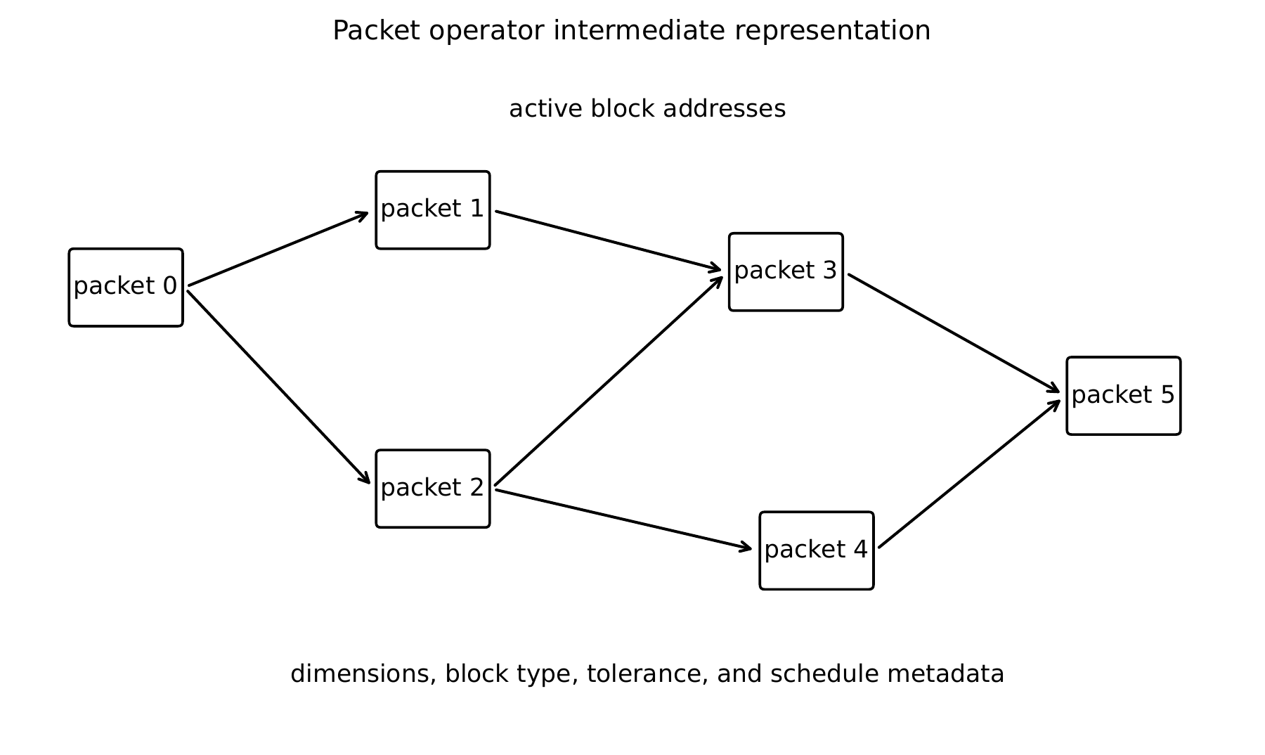
A packet intermediate representation stores active block addresses together with dimensions, block types, tolerances, and scheduling metadata.

Theorem 2.5: Block composition

Let \(A,B\in{\operatorname{End}}(X)\). Then

\[ \boxed{ (AB)_{\gamma\alpha} = \sum_{\beta\in I} A_{\gamma\beta}B_{\beta\alpha}. } \]

Consequently,

\[ {\operatorname{supp}}(AB) \subseteq {\operatorname{supp}}(A)\circ{\operatorname{supp}}(B), \]

where relational composition is defined by

\[ (\gamma,\alpha)\in E\circ F \]

when some \(\beta\) satisfies

\[ (\gamma,\beta)\in E, \qquad (\beta,\alpha)\in F. \]

Read proof · Visual guide: Two routes can cancel exactly · Read statement and proof side by side · Permalink · Source line 152 · Claim record · Lean coverage · Code · Worked examples

Proof of Theorem 2.5

Insert the packet identity between \(A\) and \(B\):

\[ P_\gamma ABP_\alpha = \sum_\beta P_\gamma AP_\beta BP_\alpha. \]

A summand can be nonzero only when both block addresses are active.

Back to statement · Read statement and proof side by side · Permalink · Source line 180 · Claim record · Lean coverage · Code · Worked examples

Corollary 2.6: Adjoint and tensor semantics

The adjoint representation has blocks

\[ (A^*)_{\alpha\beta}=A_{\beta\alpha}^*. \]

If \(A\) and \(B\) are packet resolved on \(X\) and \(Y\), then

\[ (A\otimes B)_{(\beta,\delta),(\alpha,\gamma)} = A_{\beta\alpha}\otimes B_{\delta\gamma}. \]

Read proof · Read statement and proof side by side · Permalink · Source line 191 · Claim record · Lean coverage · Code · Worked examples

Proof of Corollary 2.6

Both identities follow by inserting the corresponding coordinate projectors and using

\[ (P_\beta AP_\alpha)^*=P_\alpha A^*P_\beta. \]

The tensor identity follows from

\[ (P_\beta\otimes Q_\delta) (A\otimes B) (P_\alpha\otimes Q_\gamma) = A_{\beta\alpha}\otimes B_{\delta\gamma}. \]

Back to statement · Read statement and proof side by side · Permalink · Source line 204 · Claim record · Lean coverage · Code · Worked examples

2.2 Output contracts

On this page · Permalink · Source line 219

Definition 2.7: Output contract

An output contract specifies the mathematical object returned by an algorithm. The contract may require an explicit vector, an explicit matrix, block factors, low rank factors, spectral factors, or an implicit operator with a declared application rule.

Visual guide: The objects and their contracts · Permalink · Source line 221 · Claim record · Lean coverage · Code · Worked examples

Definition 2.8: Timing scope

A timing scope states which costs are included. Possible costs include structure discovery, compilation, host transfer, device transfer, kernel execution, graph capture, graph replay, factor reconstruction, and explicit materialization.

Permalink · Source line 225 · Claim record · Lean coverage · Code · Worked examples

Proposition 2.9: Contract conversion

Suppose one algorithm returns a compressed representation \(R\) and another returns an explicit object \(Y\). A direct timing comparison is valid only if

\[ \operatorname{decode}(R)=Y \]

and the time required by \(\operatorname{decode}\) is included, or if the downstream task consumes \(R\) directly.

Read proof · Visual guide: Same output before comparing times · Read statement and proof side by side · Permalink · Source line 229 · Claim record · Lean coverage · Code · Worked examples

Proof of Proposition 2.9

Without decoding, the two procedures return different mathematical objects. A timing ratio between different outputs does not compare implementations of the same map. Including the decoding cost gives two procedures with the same output. If the next operation consumes \(R\), decoding is not part of the declared computation.

Back to statement · Read statement and proof side by side · Permalink · Source line 237 · Claim record · Lean coverage · Code · Worked examples

Remark 2.10

A compressed product and an explicit matrix product may both be exact. They still have different contracts. This distinction becomes decisive when materialization costs \(n^2\) entries.

Permalink · Source line 241

Source and conversion record

Source SHA-256: ef616bca9291ac766d492b88f3166be4bc2b39f9ba6034dea3a4bcf2d2bf5d7f

Unsupported prose commands stop the build. The mathematical expression sequence is checked against the source, with manuscript macros expanded for display.

Conversion records

Read and explore

Proofs and implementation

About this work

Other resources