
Take \(c=(2,1,0,-1)^T\) and define \(C(c)_{jk}=c_{j-k\bmod4}\). The unitary Fourier matrix is \(F_{jk}=\mathrm i^{-jk}/2\). Its normalization is visible in the exact diagonalization:
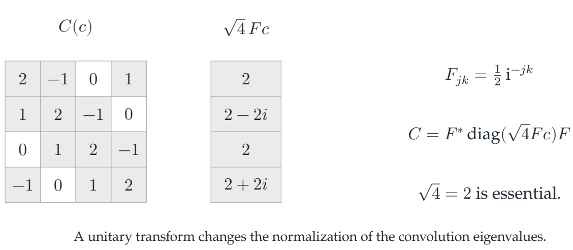
Reading the drawing
The displayed finite arrays retain the cyclic boundary convention and exact coefficients. A structured representation changes the calculation without changing the requested map.
Drawing labels and data 26 labels
Read the original labels as selectable text. Tables preserve grid relationships; other short labels are grouped compactly.
- \(C(c)\)
| Row / column | Column 1 | Column 2 | Column 3 | Column 4 |
|---|---|---|---|---|
| Row 1 | \(2\) | \(-1\) | \(0\) | \(1\) |
| Row 2 | \(1\) | \(2\) | \(-1\) | \(0\) |
| Row 3 | \(0\) | \(1\) | \(2\) | \(-1\) |
| Row 4 | \(-1\) | \(0\) | \(1\) | \(2\) |
- \(\sqrt4\,Fc\)
- \(2\)
- \(2 - 2 i\)
- \(2\)
- \(2 + 2 i\)
\(F_{jk}=\frac12\,\mathrm i^{-jk}\)
- \(C=F^*{\operatorname{diag}}(\sqrt4 Fc)F\)
- \(\sqrt4=2\) is essential.
A unitary transform changes the normalization of the convolution eigenvalues.
Follow an actual input
For \(x=(1,2,-1,0)^T\), dense multiplication gives \((0,6,0,-2)^T\). Transforming \(x\), multiplying by the four displayed eigenvalues, and applying \(F^*\) gives exactly the same vector. Every entry belongs to \({\mathbb Q}(\mathrm i)\), so the check needs no approximate trigonometric values.
There is a common normalization trap. With an unnormalized discrete transform, the convolution multiplier has one convention. With the unitary transform used here, the eigenvalue vector is \(\sqrt n\,Fc\), not \(Fc\). Dropping the factor two reconstructs \(C/2\) rather than \(C\) in this example. The invalid control deliberately tries that change and rejects it.
Where the fast algorithm enters
The identity specifies the represented operator. An FFT is an additional factorization that evaluates the transforms efficiently. The algebraic diagonalization does not certify a particular floating-point FFT, data layout, or launch policy. For a tiny four-point example, direct multiplication may be the simpler execution path even though the frequency representation is exact.
Read this as
Transform coordinates change both the storage pattern and the normalization conventions. Verify the inverse transform and convolution scale before interpreting a frequency-domain product.