
Take sensitivities \(s=(1,2,4)\), cost coefficients \(c=(1,1,2)\), and budget \(\tau=1\). Minimizing \(\sum_ec_e\log(1/\epsilon_e)\) subject to \(\sum_es_e\epsilon_e=1\) gives
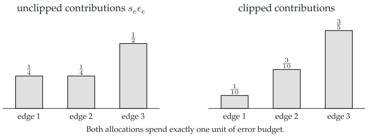
Reading the drawing
The plotted allocation follows the declared error model and cost data. Bounds on allowable choices clip the continuous solution and must remain part of the optimization.
Drawing labels and data 15 labels
Read the original labels as selectable text. Tables preserve grid relationships; other short labels are grouped compactly.
- unclipped contributions \(s_e\epsilon_e\)
- edge 1
\(\frac{1}{4}\)
- edge 2
\(\frac{1}{4}\)
- edge 3
\(\frac{1}{2}\)
- clipped contributions
- edge 1
\(\frac{1}{10}\)
- edge 2
\(\frac{3}{10}\)
- edge 3
\(\frac{3}{5}\)
Both allocations spend exactly one unit of error budget.
The budget is weighted
The three contributions to the error allowance are \((1/4,1/4,1/2)\). Equal cost coefficients give equal weighted contributions, not equal tolerances. The third edge has twice the cost coefficient of the second, which offsets its doubled sensitivity in this example.
Now impose upper tolerances \(m=(1/10,1/2,1/2)\). The first edge must stop at its tighter cap. With multiplier \(\lambda=10/3\), the clipped solution is
Its weighted contributions are \((1/10,3/10,3/5)\) and still sum to one. The checker verifies the active cap, the multiplier equations, and the budget exactly.
From tolerance to a real data type
The continuous objective is a model. Actual kernels offer discrete precisions and may use different accumulation types. A tolerance below one does not identify a particular hardware format. The finite option program on the next page is the correct next step once admissible costs and error bounds have been supplied.
Read this as
Precision allocation is an optimization over certified sensitivities and costs. It does not infer error bounds from a data-type name alone.