
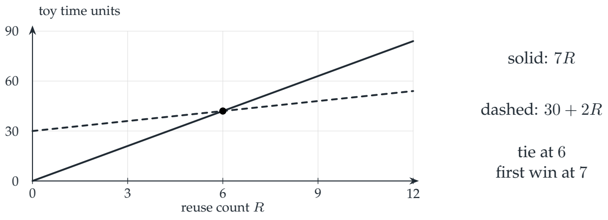
Suppose the baseline costs seven units per use. A candidate costs 30 units to set up and two per use. These are synthetic constants chosen to expose the exact threshold:
Reading the drawing
The two affine cost models are compared at integer reuse counts. A tie is separate from the first strict win; these lines are modeled costs rather than timings.
Drawing labels and data 14 labels
Read the original labels as selectable text. Tables preserve grid relationships; other short labels are grouped compactly.
- 0
- 3
- 6
- 9
- 12
- 0
- 30
- 60
- 90
- reuse count \(R\)
- toy time units
- solid: \(7R\)
- dashed: \(30+2R\)
tie at \(6\)
first win at \(7\)
At \(R=6\), both cost 42. The candidate becomes strictly faster at \(R=7\), where it costs 44 instead of 49. The minimum profitable integer reuse count is
Replacing the floor-plus-one rule with a ceiling would be wrong when the ratio is already an integer and strict improvement is required.
Which costs belong to setup?
Discovery, compilation, host/device transfer, graph capture, and factor preparation can have different reuse lifetimes. If a matrix changes but its shape does not, a captured schedule might remain reusable while its numerical factors do not. A single setup number is meaningful only after those lifetimes are fixed.
Materialization has the opposite tradeoff: pay once for an explicit representation, then use a potentially faster dense downstream operation. It pays off only when the explicit per-use cost is lower and the reuse count exceeds the corresponding conversion threshold.
Read this as
A faster steady-state kernel can lose end-to-end. State the reuse regime and count the tie separately from the first strict win.