
Let
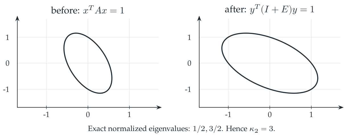
Then \(BAB=I+E={\begin{pmatrix}1&1/2\\1/2&1\end{pmatrix}}\). Its exact eigenvalues are \(1/2\) and \(3/2\), giving condition number three.
Reading the drawing
The displayed normalization separates the block diagonal part from the residual coupling. The estimate is tied to the specified operator norm and hypotheses.
Drawing labels and data 15 labels
Read the original labels as selectable text. Tables preserve grid relationships; other short labels are grouped compactly.
- -1
- 0
- 1
- -1
- 0
- 1
- before: \(x^TAx=1\)
- -1
- 0
- 1
- -1
- 0
- 1
- after: \(y^T(I+E)y=1\)
Exact normalized eigenvalues: \(1/2,3/2\). Hence \(\kappa_2=3\).
The unit circles of the energy norms
The left ellipse is \(x^TAx=1\). Writing \(x=By\) gives the right ellipse \(y^T(BAB)y=1\). The drawing samples these explicitly defined curves; the norm and eigenvalue equalities are checked symbolically.
Here \(\|E\|_2=1/2\). The manuscript's general inequality
is attained. The raw off-diagonal entry is one; its meaningful size is one-half only after normalization by the diagonal energy scales.
Keep the convergence input separate
The condition bound can be inserted into a conjugate-gradient convergence estimate under that method's positive-definite assumptions. The CG estimate is one of the separately tracked classical inputs. The algebraic normalization theorem does not certify every stopping rule, floating-point iteration, or arbitrary preconditioner.
Read this as
A small raw coupling is not scale-invariant. Normalize against the diagonal blocks before deciding whether the coupling is weak enough for a condition bound.