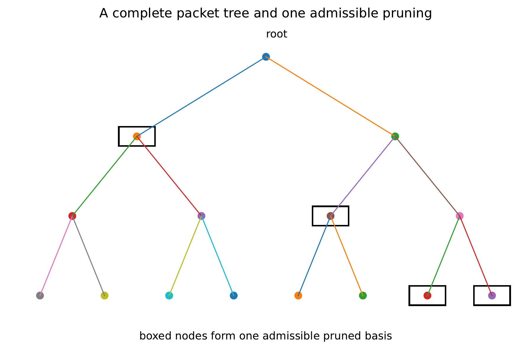
Paper V: Wavelet packet trees and admissible bases

E6 Wavelet packet trees and admissible bases

On this page · Permalink · Source line 2328

A packet transform is built by deciding at each node whether to retain the current coordinate space or to split it into children. The proof of reconstruction is local and does not depend on a particular wavelet family.

Permalink · Source line 2330

Definition E6.1: Unitary packet tree

A finite unitary packet tree consists of Hilbert spaces \({\mathcal H}_v\) at its vertices and, at every internal vertex \(v\), a unitary map

\[ U_v:{\mathcal H}_v\longrightarrow\bigoplus_{w\in\operatorname{child}(v)}{\mathcal H}_w. \]

An admissible pruning is a set of vertices that meets every root to terminal path exactly once.

Permalink · Source line 2332 · Claim record · Lean coverage · Code · Worked examples

Theorem E6.2: Reconstruction on a pruned packet tree

Every admissible pruning \({\mathcal L}\) defines a unitary analysis map

\[ {\mathcal A}_{{\mathcal L}}:{\mathcal H}_{\rm root} \longrightarrow \bigoplus_{v\in{\mathcal L}}{\mathcal H}_v. \]

Its inverse is obtained by applying the adjoints of the local splits from the leaves toward the root. In particular,

\[ \|x\|^2 = \sum_{v\in{\mathcal L}}\|x_v\|^2. \]

Read proof · Read statement and proof side by side · Permalink · Source line 2340 · Claim record · Lean coverage · Code · Worked examples

Proof of Theorem E6.2

Proceed by induction on the depth of the retained subtree. If the root is retained, the statement is immediate. If the root is split, apply the unitary map \(U_{\rm root}\), then apply the induction hypothesis independently in each child subtree. A direct sum of unitary maps is unitary. Reversing the maps with adjoints gives synthesis.

Back to statement · Read statement and proof side by side · Permalink · Source line 2355 · Claim record · Lean coverage · Code · Worked examples

Corollary E6.3: Coefficient perturbations in a unitary tree

Let \(c={\mathcal A}_{{\mathcal L}}x\) be the leaf coefficients of an admissible unitary pruning, and let \(\widehat c=c+e\). If \(\widehat x\) is synthesized from \(\widehat c\), then

\[ \|\widehat x-x\|=\|e\|. \]

Thus coefficient quantization and coefficient noise are neither amplified nor attenuated by exact unitary synthesis.

Read proof · Read statement and proof side by side · Permalink · Source line 2359 · Claim record · Lean coverage · Code · Worked examples

Proof of Corollary E6.3

The synthesis map is unitary by Theorem E6.2. Hence

\[ \widehat x-x ={\mathcal A}_{{\mathcal L}}^{-1}e \]

has the same norm as \(e\).

Back to statement · Read statement and proof side by side · Permalink · Source line 2367 · Claim record · Lean coverage · Code · Worked examples

Proposition E6.4: Bounds for nonunitary local splits

Suppose every internal node has an analysis map \(U_v\) and constants \(0\leq A_v\leq B_v<\infty\) satisfying

\[ A_v\|x\|^2 \leq \sum_{w\in\operatorname{child}(v)}\|(U_vx)_w\|^2 \leq B_v\|x\|^2. \]

Define recursively

\[ a(v)= \begin{cases} 1,&v\text{ retained},\\ A_v\min_w a(w),&v\text{ split}, \end{cases} \]

and

\[ b(v)= \begin{cases} 1,&v\text{ retained},\\ B_v\max_w b(w),&v\text{ split}. \end{cases} \]

Then the leaf analysis of the pruned tree has bounds \(a({\rm root})\) and \(b({\rm root})\).

Read proof · Visual guide: Nonunitary tree bounds propagate along branches · Read statement and proof side by side · Permalink · Source line 2376 · Claim record · Lean coverage · Code · Worked examples

Proof of Proposition E6.4

Assume the child subtree bounds have been proved. Then

\[ \sum_{w}\sum_{\ell\in{\mathcal L}_w}\|x_\ell\|^2 \geq \min_w a(w) \sum_w\|(U_vx)_w\|^2 \geq A_v\min_w a(w)\|x\|^2. \]

The upper bound follows in the same way with the maximum and \(B_v\). Induction completes the proof.

Back to statement · Read statement and proof side by side · Permalink · Source line 2404 · Claim record · Lean coverage · Code · Worked examples

A complete wavelet packet tree and an admissible pruning at mixed depths. — A complete packet tree and one admissible pruning. Retained nodes may occur at different depths.

E6.1 Best basis recursion

On this page · Permalink · Source line 2424

The minimum is taken over feasible prunings

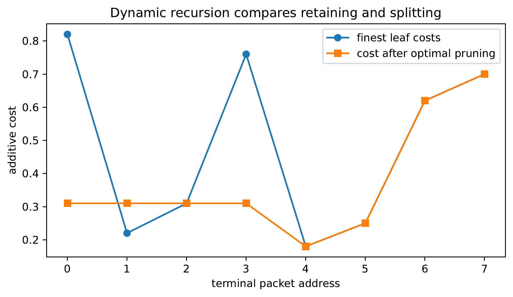
The value at a node is the least cost among all admissible prunings of the subtree rooted there. It is one optimal value. Individual competing prunings may have larger costs. The recursion compares retaining the node with the sum of the already optimal child values, with retention chosen on a tie.

Permalink · Source line 2426

Assign a real cost \(c(v)\) to retaining each node. For an admissible pruning \({\mathcal L}\), let

\[ C({\mathcal L})=\sum_{v\in{\mathcal L}}c(v). \]

The cost may measure entropy, coefficient count, an approximation penalty, or any other additive local objective.

Permalink · Source line 2430

Theorem E6.5: Exact additive best basis recursion

For each vertex define

\[ F(v) = \min\left\{ c(v), \sum_{w\in\operatorname{child}(v)}F(w) \right\}, \]

with \(F(v)=c(v)\) at terminal vertices. Then \(F(v)\) is the minimum cost of every admissible pruning of the subtree rooted at \(v\). A minimizing pruning is recovered by retaining \(v\) when the first term is no larger than the second and splitting it otherwise.

Read proof · Read statement and proof side by side · Permalink · Source line 2436 · Claim record · Lean coverage · Code · Worked examples

Proof of Theorem E6.5

Every admissible pruning of the subtree has exactly two forms. It either retains \(v\), with cost \(c(v)\), or splits \(v\) and independently chooses an admissible pruning in every child subtree. The minimum in the second case is the sum of the child minima. This gives the recursion and the reconstruction rule. In an equality case both choices minimize, and the stated rule retains the node.

Back to statement · Read statement and proof side by side · Permalink · Source line 2449 · Claim record · Lean coverage · Code · Worked examples

Theorem E6.6: Stability of the optimal cost

Let \(c\) and \(\widetilde c\) be two node cost functions. For an admissible pruning \({\mathcal L}\), set

\[ \varepsilon({\mathcal L}) = \sum_{v\in{\mathcal L}}|c(v)-\widetilde c(v)| \]

and let

\[ \varepsilon_* = \max_{{\mathcal L}}\varepsilon({\mathcal L}). \]

If \(F_*\) and \(\widetilde F_*\) are the two optimal root costs, then

\[ |F_*-\widetilde F_*| \leq \varepsilon_*. \]

Read proof · Read statement and proof side by side · Permalink · Source line 2453 · Claim record · Lean coverage · Code · Worked examples

Proof of Theorem E6.6

For every admissible pruning,

\[ |C({\mathcal L})-\widetilde C({\mathcal L})| \leq \varepsilon_*. \]

Evaluate \(\widetilde C\) on a minimizer for \(C\) to obtain \(\widetilde F_*\leq F_*+\varepsilon_*\). Reverse the roles to obtain \(F_*\leq\widetilde F_*+\varepsilon_*\).

Back to statement · Read statement and proof side by side · Permalink · Source line 2474 · Claim record · Lean coverage · Code · Worked examples

Corollary E6.7: Stability of the selected basis

Assume the optimal pruning \({\mathcal L}_*\) for \(c\) is unique and at least one competing pruning exists. Define \(g=\min_{{\mathcal L}\ne{\mathcal L}_*}(C({\mathcal L})-C({\mathcal L}_*))>0\). If

\[ 2\varepsilon_*<g, \]

then the optimal pruning for \(\widetilde c\) is the same. If only one admissible pruning exists, it remains selected under every cost change without a gap condition.

Read proof · Read statement and proof side by side · Permalink · Source line 2484 · Claim record · Lean coverage · Code · Worked examples

Proof of Corollary E6.7

The cost of the original minimizer can increase by at most \(\varepsilon_*\), while the cost of every competitor can decrease by at most \(\varepsilon_*\). The original gap therefore remains positive.

Back to statement · Read statement and proof side by side · Permalink · Source line 2492 · Claim record · Lean coverage · Code · Worked examples

An additive recursion compares the cost of retaining a node with splitting its children. — An additive best basis recursion compares the cost of retaining a packet with the total cost of splitting it.

Source and conversion record

Source SHA-256: 5d3c6b2e5709c37ea551eb8fd1d823e5249c5fbc411d36b806241af4df888f36

Unsupported prose commands stop the build. The mathematical expression sequence is checked against the source, with manuscript macros expanded for display.

Conversion records

Read and explore

Proofs and implementation

About this work

Other resources