
E13 Finite numerical illustrations
On this page · Permalink · Source line 3589
The figures and tables in this section are finite checks and examples. They are not substitutes for the preceding proofs. Their purpose is to show the scale and shape of the terms appearing in the exact estimates.
A fixed depth Haar packet transform and a Fourier basis were applied to the same piecewise smooth test signal. The largest coefficients were retained in each representation.
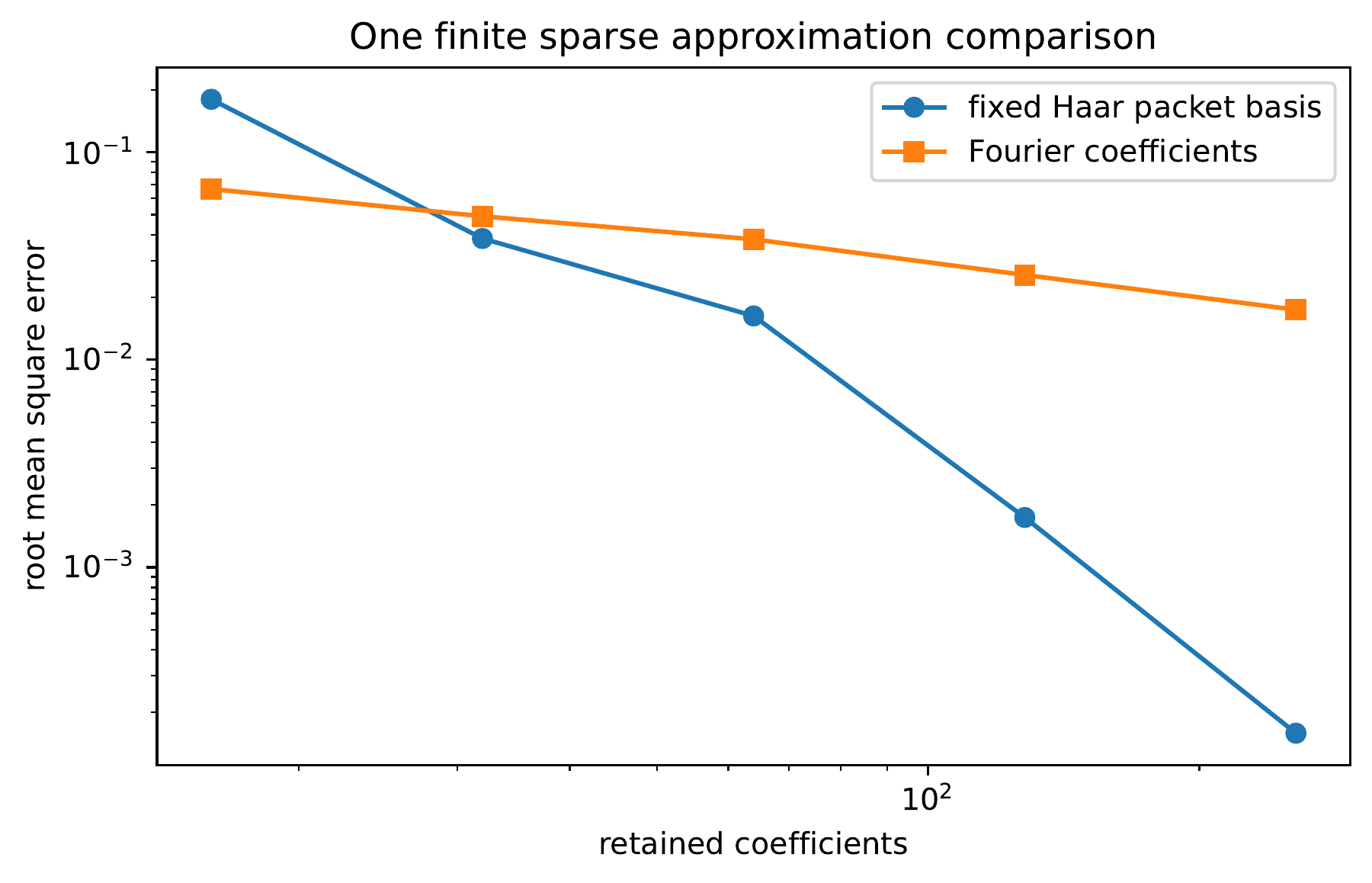
| retained | Haar packet RMSE | Fourier RMSE |
|---|---|---|
| 16 | \(1.7999\times10^{-1}\) | \(6.6522\times10^{-2}\) |
| 32 | \(3.8414\times10^{-2}\) | \(4.9153\times10^{-2}\) |
| 64 | \(1.6267\times10^{-2}\) | \(3.8056\times10^{-2}\) |
| 128 | \(1.7387\times10^{-3}\) | \(2.5631\times10^{-2}\) |
| 256 | \(1.5870\times10^{-4}\) | \(1.7424\times10^{-2}\) |
The table does not prove that Haar packets dominate Fourier coordinates for every signal. Smooth periodic oscillations may favor Fourier coordinates. Curved edges in two dimensions may favor directional systems. The geometric approximation results in [Donoho1999], [CandesDonoho2004] give much deeper statements for specific image classes.
| case | global | exact packet | estimated packet |
|---|---|---|---|
| one dimensional step | \(5.4023\times10^{-2}\) | \(1.3692\times10^{-4}\) | \(2.4029\times10^{-2}\) |
| two dimensional disk | \(3.7643\times10^{-2}\) | \(6.4752\times10^{-5}\) | \(3.4043\times10^{-3}\) |
| multiple regions | \(3.3740\times10^{-2}\) | \(5.2118\times10^{-7}\) | not evaluated |
The estimated packet rows used a narrow positive contrast synthetic model. They are not evidence for a general segmentation theorem. The exact packet rows verify Theorem E7.5 numerically after the packet is supplied.