
3 Linear time-invariant operators as transfer matrices
On this page · Permalink · Source line 407
Let \(h\) be a finite impulse response and
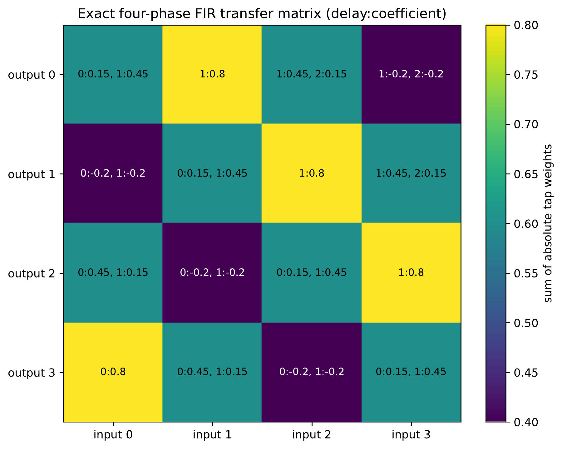
Resolve both input and output into \(N\) phases. For output phase \(k\) and input phase \(s\), define the transfer kernel
Out-of-range taps are understood to be zero.
Theorem 3.1: Exact FIR polyphase transfer law
The output channels satisfy
For the numerical channel transform, take \(z\in{\mathbb C}\setminus\{0\}\) and assume
Define \(X_s(z)=\sum_nx_s[n]z^{-n}\). The output series then also converge absolutely, and
Read proof · Visual guide: A filter becomes a matrix of actual delays · Read statement and proof side by side · Permalink · Source line 423 · Claim record · Lean coverage · Code · Worked examples
Proof of Theorem 3.1
Evaluate \(y\) at address \(Nn+k\) and partition every input index by its residue \(s\):
For a fixed output phase \(k\), the change of tap address \(q=Nm+k-s\) is a bijection between \({\mathbb Z}\) and the pairs \((s,m)\) with \(0\le s<N\): choose \(s\equiv k-q\pmod N\) and then \(m=(q-k+s)/N\). Thus this is a reindexing of the finite filter support, valid for every bilateral input sequence, without a convergence assumption on \(x\).
The last factor is \(x_s[n-m]\), giving the time-domain formula. Under the additional transform hypothesis, each delayed channel has transform
Absolute summability permits this bijective reindexing, and only finitely many delayed channels are combined. Taking their finite linear combination gives the matrix formula. The time-domain theorem therefore remains valid even when no numerical bilateral transform exists.
Back to statement · Read statement and proof side by side · Permalink · Source line 445 · Claim record · Lean coverage · Code · Worked examples
Remark 3.2: Operator-block form
If \(H\) denotes convolution by \(h\), the same identity is
Thus the familiar polyphase matrix is exactly the transfer-block matrix of the seed calculus.