
Take \(p=2\) and the supplied diagonal weights \((s_0,s_1,s_2)=(0,1,3)\). At depth \(L\), an admissible target has
Each direction contributes only the amount visible at the current depth.
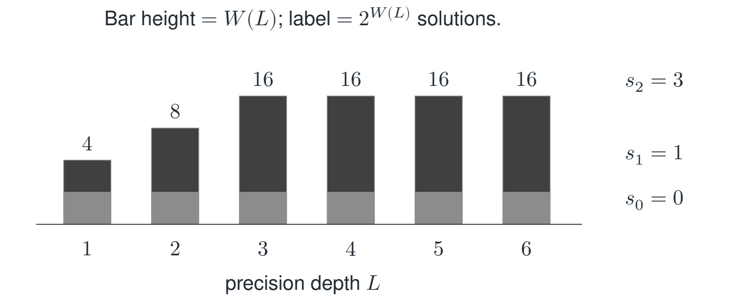
Reading the drawing
Stacked bars record the exponent of the fiber size, and the labels give the actual cardinality. Each shade belongs to one supplied directional weight.
Drawing labels and data 17 labels
Read the original labels as selectable text. Tables preserve grid relationships; other short labels are grouped compactly.
- \(4\)
- \(1\)
- \(8\)
- \(2\)
- \(16\)
- \(3\)
- \(16\)
- \(4\)
- \(16\)
- \(5\)
- \(16\)
- \(6\)
- precision depth \(L\)
- Bar height \(=W(L)\); label \(=2^{W(L)}\) solutions.
- \(s_2=3\)
- \(s_1=1\)
- \(s_0=0\)
Evidence note from the source edition
The stacked height records the exponent \(W(L)\). The label above each bar records the actual number of solutions. The zero-weight direction contributes no branching. This is a finite cardinality calculation, not an information-theoretic assumption about random inputs.
The values are
Once \(L\ge3\), the nonzero weights have been fully exposed and the admissible fiber cardinality stabilizes at sixteen. The input space still grows as \(2^{3L}\). The number of attainable targets grows accordingly.
At depth six, \((1,2,8)\) is admissible and gives sixteen solutions. Replacing the last coordinate by four makes the target inadmissible and gives zero solutions, even though the weights and depth are unchanged.
What changes with a zero diagonal factor?
A literal zero factor contributes \(L\), not a fixed eventual weight, and requires a zero target coordinate. Its fiber therefore keeps growing with the modulus. That case must not be mistaken for a finite nonzero Smith weight.
Read this as
The scalar sum of weights gives the count, but the separate weights give the admissibility conditions. Keeping only a determinant valuation can hide which target coordinate fails.