
7 Rational spectral projectors and resultant bounds
On this page · Permalink · Source line 1
Let \({{\mathcal O}}\) be a discrete valuation ring with fraction field \(K\) and uniformizer \(\pi\). Let \(\Lambda\) be a finite free \({{\mathcal O}}\) module and put
Suppose \(A\in{\operatorname{End}}_{{{\mathcal O}}}(\Lambda)\).
Theorem 7.1: Bézout spectral projector
Assume that
with monic polynomials \(f,g\in{{\mathcal O}}[x]\) that are coprime in \(K[x]\). Choose \(u,v\in{{\mathcal O}}[x]\) and a nonzero \(r\in{{\mathcal O}}\) such that
Then
is the projector of \(V\) onto \({\operatorname{Ker}} f(A)\) along \({\operatorname{Ker}} g(A)\). In particular,
Read proof · Read statement and proof side by side · Permalink · Source line 9 · Claim record · Lean coverage · Code · Worked examples
Proof of Theorem 7.1
Cayley Hamilton gives
If \(x\in{\operatorname{Ker}} f(A)\), then the Bézout identity gives
so \(E_fx=x\). If \(x\in{\operatorname{Ker}} g(A)\), then \(E_fx=0\). The same identity gives the direct sum decomposition
Indeed, every \(x\in V\) is the sum of
and
Thus \(E_f\) is the stated projector and is idempotent. The formula for \(rE_f\) has coefficients in \({{\mathcal O}}\), so it preserves \(\Lambda\).
Back to statement · Read statement and proof side by side · Permalink · Source line 30 · Claim record · Lean coverage · Code · Worked examples
Theorem 7.2: Several coprime spectral packets
Assume
where the monic factors \(f_i\in{{\mathcal O}}[x]\) are pairwise coprime in \(K[x]\). Put
There are complementary projectors \(E_i\) with
One may choose \(E_i\) so that
up to multiplication of the resultant by a unit.
Read proof · Read statement and proof side by side · Permalink · Source line 54 · Claim record · Lean coverage · Code · Worked examples
Proof of Theorem 7.2
Apply Theorem 7.1 to the factorization \(\chi_A=f_ig_i\). The resulting projector is one on \({\operatorname{Ker}} f_i(A)\) and zero on every \({\operatorname{Ker}} f_j(A)\) with \(j\ne i\). The direct sum decomposition follows from the polynomial Chinese remainder theorem. The orthogonality and sum identities follow by evaluating the corresponding idempotents in \(K[x]/(\chi_A)\). The Sylvester Bézout relation for \((f_i,g_i)\) gives the stated denominator bound.
Back to statement · Read statement and proof side by side · Permalink · Source line 79 · Claim record · Lean coverage · Code · Worked examples
Corollary 7.3: Resultant denominator bound
Under the hypotheses of Theorem 7.1, one may take
up to multiplication by a unit. Therefore
Read proof · Read statement and proof side by side · Permalink · Source line 83 · Claim record · Lean coverage · Code · Worked examples
Proof of Corollary 7.3
The Sylvester matrix construction gives a Bézout relation with right side equal to the resultant. Apply Theorem 7.1. Standard facts about resultants may be found in [Lang2002], [GohbergLancasterRodman2009].
Back to statement · Read statement and proof side by side · Permalink · Source line 94 · Claim record · Lean coverage · Code · Worked examples
Example 7.4: A resultant bound that is not exact
Let
on the standard lattice \(\Lambda={{\mathcal O}}^2\). The factors \(x\) and \(x-\pi^s\) have resultant \(-\pi^s\), up to the harmless choice of resultant order, but the two spectral projectors are the integral coordinate projectors. Their exact separation weight is zero. The resultant sees the closeness of the two eigenvalues. It does not see that the chosen lattice already splits along their eigenspaces.
How to read the result
A resultant bounds the denominator through the characteristic factors. The exact separation weight also depends on how the lattice sits inside the rational packet spaces. These are two stages of the calculation. First construct a rational projector with a known clearing denominator. Then measure the gluing of the chosen lattice to find the least denominator that actually works.
7.1 Evaluated certificates and explicit lattice action
On this page · Permalink · Source line 110
7.1.1 Minimal evaluated Bézout identities
On this page · Permalink · Source line 112
Let \({{\mathcal O}}\) be a DVR, \(K={\operatorname{Frac}}({{\mathcal O}})\), and \(A\in{\operatorname{End}}_{{\mathcal O}}(\Lambda)\) for a finite free lattice \(\Lambda\). Suppose the characteristic polynomial factors over \({{\mathcal O}}\) as
where \(f\) and \(g\) are coprime over \(K[x]\).
Theorem 7.5: Evaluated Bézout spectral projector
Let \(F,G,U,V\in{\operatorname{End}}_K(\Lambda\otimes_{{\mathcal O}} K)\) and let \(r\in K^\times\). Suppose
Put \(N=VG\). Then
Consequently the operator
is idempotent, acts as the identity on \(\ker F\), and acts as zero on \(\ker G\). If \(V\) and \(G\) preserve \(\Lambda\), then
Read proof · Visual guide: Separate before dividing · Read statement and proof side by side · Permalink · Source line 120 · Claim record · Lean coverage · Code · Worked examples
Proof of Theorem 7.5
The Bézout identity gives \(N=rI-UF\). The two stated commutation relations and \(FG=0\) give
Therefore
Since \(r\ne0\), \(E^2=r^{-2}N^2=E\). If \(Fx=0\), the evaluated Bézout identity gives \(VGx=rx\), hence \(Ex=x\). If \(Gx=0\), then \(Ex=0\). The lattice assertion follows directly from \(rE=VG\).
Back to statement · Read statement and proof side by side · Permalink · Source line 146 · Claim record · Lean coverage · Code · Worked examples
The equality \(N^2=rN\) before division uses neither \(r\ne0\) nor the other pairwise commutation relations that hold in the polynomial application. Normalizing to \(E\) uses \(r\ne0\). Its action on \(\ker F\) uses only the Bézout identity and \(r\ne0\), while vanishing on \(\ker G\) follows immediately from \(N=VG\). The bundled Lean certificate records all pairwise commutations as convenient evaluated polynomial data, but the minimal theorems expose only the hypotheses they consume.
For the polynomial application, one supplies \(F=f(A)\), \(G=g(A)\), \(U=u(A)\), and \(V=v(A)\). A Bézout or resultant identity \(uf+vg=r\) evaluates to the first certificate, while \((fg)(A)=0\) supplies the second. When \(fg=\chi_A\), this last equality is Cayley Hamilton. Standard Bézout, resultant, and DVR facts are recalled from [Lang2002], [Serre1979]. The inherited certificate theorem begins with the evaluated certificate. It does not infer exact action merely from nilpotence of \(f(A)\) or \(g(A)\), which would be insufficient.
Definition 7.6: Separation weight
For a rational projector \(E\) and a specified \({{\mathcal O}}\) lattice \(\Lambda\), provided at least one clearing exponent exists, define
If the evaluated certificate arises from integral \(v,g\) and \(r=u\pi^s\) with \(u^{-1}\) preserving the lattice, then Theorem 7.5 gives the upper bound
Indeed,
preserves \(\Lambda\). The minimal Lean theorem needs only the lattice action of \(u^{-1}\). The bundled wrapper for lattice units records both \(u\) and \(u^{-1}\). A nonzero scalar in the fraction field need not be an integral unit. Existence of a clearing exponent is an explicit hypothesis. Once one exists, the least one is obtained from the least element property of the natural numbers. Clearing exponents are upward closed provided multiplication by \(\pi\) preserves the lattice.
Visual guide: An atlas of the refinement layer · Visual guide: Separate before dividing · Permalink · Source line 178 · Claim record · Lean coverage · Code · Worked examples
7.1.2 Certificate-level precision delay
On this page · Permalink · Source line 205
Theorem 7.7: Projector precision delay
Let \(E\) be a rational projector with \(\pi^sE(\Lambda)\subseteq\Lambda\). If
then
Thus \(m+s\) input digits suffice to determine \(m\) output digits of the projected packet.
Read proof · Visual guide: Three kinds of resolution · Visual guide: One extra digit is genuinely necessary · Read statement and proof side by side · Permalink · Source line 207 · Claim record · Lean coverage · Code · Worked examples
Proof of Theorem 7.7
Write \(x-y=\pi^{m+s}z\). Since \(\pi^sE(z)\in\Lambda\),
Back to statement · Read statement and proof side by side · Permalink · Source line 219 · Claim record · Lean coverage · Code · Worked examples
The theorem gives a precision budget for delayed separation. A packet with weight \(s\) can be reconstructed at the requested output precision by retaining \(s\) additional input digits.
8 Exact lattice separation
On this page · Permalink · Source line 229
The exact denominator belongs to the pair consisting of the rational packet decomposition and the integral lattice.
Definition 8.1: Lattice packet data
Let
be a finite direct sum over \(K\), with packet projectors \(E_\alpha\). Let \(\Lambda\subseteq V\) be an \({{\mathcal O}}\) lattice. Put
and define the gluing module
The separation weight of \(E_\alpha\) is
The global separation weight is
For a finitely generated torsion \({{\mathcal O}}\) module \(G\), write \({\operatorname{exp}}_\pi(G)\) for the least \(s\) such that \(\pi^sG=0\).
Permalink · Source line 234 · Claim record · Lean coverage · Code · Worked examples
The gluing module \(G_{\Lambda,{\mathcal P}}\) is a finitely generated torsion \({{\mathcal O}}\) module, hence has finite length, because \(\Lambda_{\mathrm{split}}\) and \(\Lambda\) are full lattices in the same vector space. To see that the split lattice is full, clear denominators of bases of the rational summands. Each \(\Lambda\cap V_\alpha\) then spans \(V_\alpha\), so their direct sum spans \(V\).
Theorem 8.2: Gluing module and exact separation weight
With the notation of Definition 8.1, the map
is injective, and every coordinate projection of its image is surjective. We also have
If
with \(a_1\leq\cdots\leq a_r\), then
Read proof · Read statement and proof side by side · Permalink · Source line 266 · Claim record · Lean coverage · Code · Worked examples
Proof of Theorem 8.2
If \(x\in\Lambda\) maps to zero, then \(E_\alpha x\in\Lambda_\alpha\) for every \(\alpha\). Since
we have \(x\in\Lambda_{\mathrm{split}}\). Thus \(\Phi\) is injective. The coordinate map onto \(E_\alpha\Lambda/\Lambda_\alpha\) is surjective by the definition of \(E_\alpha\Lambda\).
Let \(s=s_\Lambda({\mathcal P})\). For every \(x\in\Lambda\) and every \(\alpha\),
Hence
so \(\pi^sG_{\Lambda,{\mathcal P}}=0\). This proves
If \(d<s\), then for some \(\alpha\) there is an \(x\in\Lambda\) with
The class \(\pi^d[x]\) is therefore nonzero in the gluing module. Thus \(\pi^d\) does not annihilate the gluing module, and equality follows. The final formula is the usual description of the exponent through Smith normal form.
Back to statement · Read statement and proof side by side · Permalink · Source line 295 · Claim record · Lean coverage · Code · Worked examples
Corollary 8.3: Total gluing and worst precision
If
then
Thus the lattice index measures the total amount of gluing, while the separation weight measures the worst precision loss in one direction.
Read proof · Read statement and proof side by side · Permalink · Source line 321 · Claim record · Lean coverage · Code · Worked examples
Proof of Corollary 8.3
The length and exponent of a finitely generated torsion module are read directly from its Smith decomposition. Apply Theorem 8.2.
Back to statement · Read statement and proof side by side · Permalink · Source line 339 · Claim record · Lean coverage · Code · Worked examples
Corollary 8.4: Two complementary packets
Suppose
with projector \(E\) onto \(V_1\) and complementary projector \(I-E\). Then
Consequently
Read proof · Read statement and proof side by side · Permalink · Source line 343 · Claim record · Lean coverage · Code · Worked examples
Proof of Corollary 8.4
Map \(x\in\Lambda\) to \(Ex+\Lambda_1\). Its kernel consists of the \(x\) for which \(Ex\in\Lambda_1\). In that case
so the kernel is \(\Lambda_1\oplus\Lambda_2\). The map is surjective by definition. The complementary map is handled in the same way. The equality of weights follows from Theorem 8.2.
Back to statement · Read statement and proof side by side · Permalink · Source line 364 · Claim record · Lean coverage · Code · Worked examples
Corollary 8.5: Integral splitting criterion
Every packet projector preserves \(\Lambda\) if and only if
Equivalently,
Read proof · Read statement and proof side by side · Permalink · Source line 372 · Claim record · Lean coverage · Code · Worked examples
Proof of Corollary 8.5
If every projector preserves \(\Lambda\), then
expresses every \(x\in\Lambda\) as a sum of vectors in \(\Lambda_\alpha\). The converse is immediate because each projector is the identity on one direct summand and zero on the others. The final equivalence follows from Theorem 8.2.
Back to statement · Read statement and proof side by side · Permalink · Source line 385 · Claim record · Lean coverage · Code · Worked examples
8.1 Refinement and separation weight
On this page · Permalink · Source line 393
A finer rational packet system imposes more integral splitting conditions.
Theorem 8.6: Gluing exact sequence under refinement
Let \({\mathcal Q}=(Q_\beta)\) refine \({\mathcal P}=(P_\alpha)\) on \(V\), and let \(\Lambda\) be a lattice. Define
Then
and there is a short exact sequence
In particular,
Read proof · Read statement and proof side by side · Permalink · Source line 397 · Claim record · Lean coverage · Code · Worked examples
Proof of Theorem 8.6
Every fine packet space lies in its parent packet space, so every element of \(\Lambda_{{\mathcal Q}}\) belongs to \(\Lambda_{{\mathcal P}}\). The displayed exact sequence is the standard quotient sequence for nested submodules. The exponent of a quotient cannot exceed the exponent of the module from which it is obtained. Apply Theorem 8.2 to the two gluing modules.
Back to statement · Read statement and proof side by side · Permalink · Source line 431 · Claim record · Lean coverage · Code · Worked examples
Example 8.7: Strict growth under refinement
Take the standard lattice \(\mathbb Z_2^2\) and the involution from Proposition 9.1. The one packet system \((I)\) has weight zero. Refining it into the two rational sign packets produces weight one. The coarse lattice is already split because there is only one summand. The fine eigenspaces are glued together by one dyadic digit.
Remark 8.8: Strict growth can occur
A coarse packet family may preserve the lattice even though a fine spectral split does not. Refinement can reveal rational directions that are glued together integrally. The weight records the extra depth needed to separate them.
8.2 Exact precision delay
On this page · Permalink · Source line 443
The separation weight has an operational meaning. It is the exact number of extra input digits needed to recover a projected packet uniformly.
Theorem 8.9: Necessary and sufficient precision delay
Let \(E\) be a rational projector on \(V\), let \(\Lambda\) be a lattice, and let
For every \(m\geq0\), the rule
from \(\Lambda/\pi^{m+s}\Lambda\) to \(V/\pi^m\Lambda\) is well defined. Here \(m\) is an integer. If \(d\) is an integer with \(0\leq d<s\), then for every integer \(m\geq0\) there are \(x,y\in\Lambda\) such that
but
Thus \(s\) extra digits are both sufficient and necessary for a uniform precision guarantee.
Read proof · Read statement and proof side by side · Permalink · Source line 450 · Claim record · Lean coverage · Code · Worked examples
Proof of Theorem 8.9
If
then
This proves that the rule is well defined. Now take \(d<s\). By the minimality of \(s\), there is a \(z\in\Lambda\) with
Set
Then \(x\equiv y\) modulo \(\pi^{m+d}\Lambda\), while
Back to statement · Read statement and proof side by side · Permalink · Source line 470 · Claim record · Lean coverage · Code · Worked examples
The central idea
The necessity statement is uniform over the lattice. A particular input may need fewer extra digits, but a smaller delay cannot recover every projected packet at the prescribed precision. This is why the least clearing exponent gives an exact precision guarantee rather than only a sufficient budget.
Example 8.10: The same rational split with two lattices
Let
and let \(E\) project onto \(Ke_1\). On the split lattice
the weight is zero. Fix \(s\geq1\) and consider
Then
The gluing module is isomorphic to \({{\mathcal O}}/\pi^s{{\mathcal O}}\), so
The rational decomposition has not changed. Only the lattice has changed.
The example can be realized by an integral operator. Define
In the basis
the matrix of \(A\) is
Its eigenvalue factors have resultant equal to \(\pi^s\) up to a unit, and the exact projector weight on \(\Lambda_s\) is also \(s\).
9 The dyadic sign split
On this page · Permalink · Source line 549
The smallest example already shows why coefficient selectors and spectral averages must be kept distinct.
Proposition 9.1: Sign projectors over a lattice
Let
act on \(\mathbb Z_p^2\). Over \(\mathbb Q_p\), the sign projectors are
For every odd prime \(p\), both projectors preserve \(\mathbb Z_p^2\). At \(p=2\),
The factors \(x-1\) and \(x+1\) have resultant \(2\).
Read proof · Read statement and proof side by side · Permalink · Source line 553 · Claim record · Lean coverage · Code · Worked examples
Proof of Proposition 9.1
The displayed matrices are complementary idempotents. The scalar \(2\) is a unit in \(\mathbb Z_p\) for odd \(p\), so both matrices are integral there. Over \(\mathbb Z_2\), multiplying by \(2\) clears the denominators, while neither projector preserves the standard lattice. Thus both weights are one. The resultant of the two linear factors is their root difference, which is \(2\).
Back to statement · Read statement and proof side by side · Permalink · Source line 586 · Claim record · Lean coverage · Code · Worked examples
Modulo \(2\), the two eigenvalues become equal. The rational sign packets remain distinct over \(\mathbb Q_2\), but the standard lattice does not split into their intersections until one more dyadic digit is retained.
Proposition 9.2: Integral character averages away from the group order
Let \({{\mathcal O}}\) be a discrete valuation ring, let \(N\) be a unit in \({{\mathcal O}}\), and suppose \({{\mathcal O}}\) contains a primitive \(N\)th root of unity \(\omega\). If an integral operator \(U\) satisfies \(U^N=I\), then
preserves every \(U\) stable \({{\mathcal O}}\) lattice. At primes dividing \(N\), this formula alone gives no integral projector.
Read proof · Read statement and proof side by side · Permalink · Source line 593 · Claim record · Lean coverage · Code · Worked examples
Proof of Proposition 9.2
Every scalar coefficient in the displayed sum belongs to \({{\mathcal O}}\) because \(N\) is a unit and \(\omega\) is integral. Each power of \(U\) preserves the lattice, so their \({{\mathcal O}}\) linear combination does as well. When \(N\) is not a unit, division by \(N\) is not an operation in \({{\mathcal O}}\), so the same argument is unavailable.
Back to statement · Read statement and proof side by side · Permalink · Source line 601 · Claim record · Lean coverage · Code · Worked examples
At a prime dividing \(N\), the factor \(1/N\) no longer guarantees that the character average preserves the lattice. Cancellation may still make a particular projector integral. Coefficient residue selectors remain exact because they never divide by the group order.
9.1 The concrete rational sign matrix
On this page · Permalink · Source line 607
Consider the integral involution
Over a field of characteristic different from two, its sign projectors are
They are orthogonal idempotents and sum to \(I\).
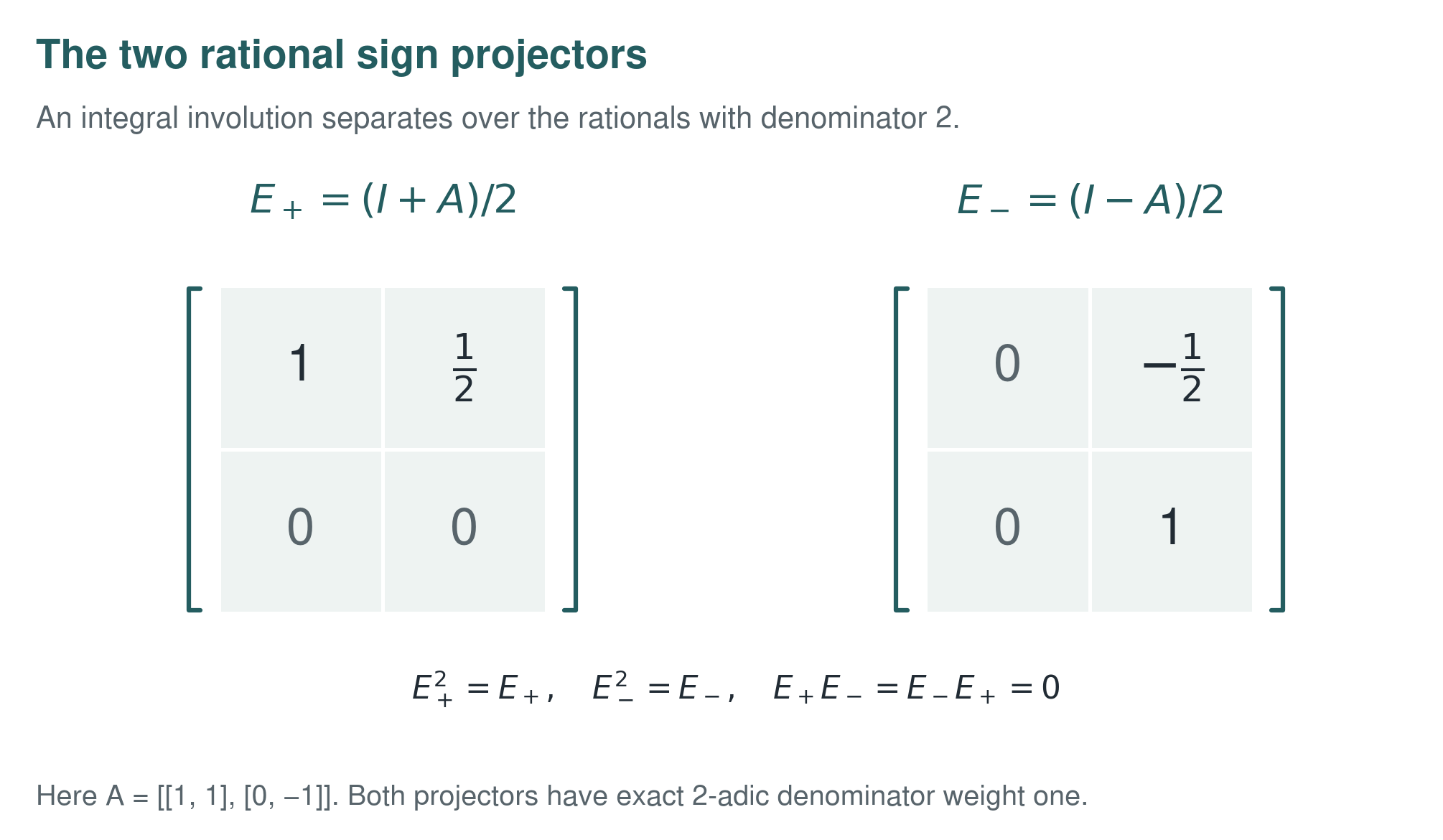
Proposition 9.3: Odd-adic versus dyadic behavior
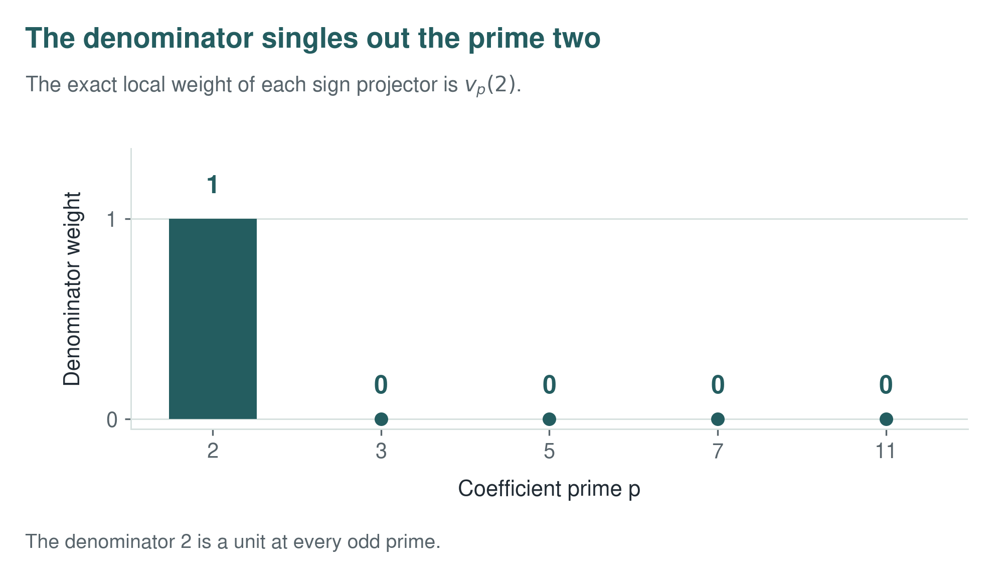
For every prime \(p\ne2\), every entry of \(E_+\) and \(E_-\) is \(p\)-integral, and each projector has exact local denominator weight zero. At \(p=2\), each projector has exact local denominator weight one. Multiplication by \(2\) makes it integral, while the unscaled matrix is not integral:
The characteristic factors \(x-1\) and \(x+1\) have resultant \(2\). Its \(2\)-adic valuation is one, exactly the two local projector weights above, and its \(p\)-adic valuation is zero at every prime \(p\ne2\).
Read proof · Visual guide: Where the dyadic digit is lost · Visual guide: One extra digit is genuinely necessary · Read statement and proof side by side · Permalink · Source line 645 · Claim record · Lean coverage · Code · Worked examples
Proof of Proposition 9.3
The reduced denominators of the displayed entries are \(1\) or \(2\), which proves the local integrality and minimality statements directly. The resultant is
Thus \(v_2(2)=1\) and \(v_p(2)=0\) for primes \(p\ne2\).
Back to statement · Read statement and proof side by side · Permalink · Source line 658 · Claim record · Lean coverage · Code · Worked examples
The two characteristic factors \(x-1\) and \(x+1\) have the same reduction in \({\mathbb F}_2[x]\). The rational matrices \(E_+\) and \(E_-\) themselves cannot be reduced modulo \(2\), because their entries contain \(1/2\). Consequently the integral special fibre does not inherit their separate idempotent splitting, even though the two projectors remain distinct over \({\mathbb Q}_2\). This is the simplest model of delayed dyadic separation.
9.1.1 Why coefficient packets remain available
On this page · Permalink · Source line 682
The failure of the character formula
to be integral does not invalidate coefficient selectors such as even and odd residue extraction. It shows that two distinct constructions must be distinguished:
when the group order is not a unit. The first can remain exact over \({\mathbb Z}_2\). The second can acquire a denominator weight.
10 Smith normal form and congruence lifting
On this page · Permalink · Source line 699
The gluing module gives the exact common denominator of packet projectors. Smith normal form gives the corresponding coordinate by coordinate solvability and branching rule.
Standard fact 10.1: Smith normal form over a discrete valuation ring
Let \(M\in M_{m,n}({{\mathcal O}})\). There are invertible matrices
such that
where
and \(r\) is the rank over \(K\). The exponents are uniquely determined. See [Newman1972].
Permalink · Source line 703 · Claim record · Lean coverage · Code · Worked examples
Proposition 10.2: Computing a packet weight from an inclusion matrix
Choose an \({{\mathcal O}}\) basis of \(\Lambda\) and an \({{\mathcal O}}\) basis of \(\Lambda_{\mathrm{split}}\). Let \(B\) be the matrix of the inclusion
If the Smith form of \(B\) is
then
Read proof · Read statement and proof side by side · Permalink · Source line 723 · Claim record · Lean coverage · Code · Worked examples
Proof of Proposition 10.2
The gluing module is the cokernel of the inclusion matrix \(B\). Smith normal form gives its invariant factors. The weight formula follows from Theorem 8.2.
Back to statement · Read statement and proof side by side · Permalink · Source line 744 · Claim record · Lean coverage · Code · Worked examples
Theorem 10.3: Smith weighted congruence solve
Let \(M\in M_{m,n}({{\mathcal O}})\) have Smith exponents \(s_1,\ldots,s_r\). Assume the residue field is finite of cardinality \(q\), fix \(L\geq1\), and consider
Put
for a Smith matrix \(U\) as in Standard fact 10.1. The congruence is solvable if and only if
and
When it is solvable, the number of solutions in \(({{\mathcal O}}/\pi^L{{\mathcal O}})^n\) is
Read proof · Read statement and proof side by side · Permalink · Source line 748 · Claim record · Lean coverage · Code · Worked examples
Proof of Theorem 10.3
Set \(x=Vy\). Multiplying the congruence by \(U\) reduces it to independent equations
and zero equations in the remaining rows. Multiplication by \(\pi^{s_i}\) on \({{\mathcal O}}/\pi^L{{\mathcal O}}\) has image equal to the elements divisible by \(\pi^{\min(s_i,L)}\) and kernel of size
Each of the \(n-r\) unused variables is free and contributes \(q^L\) choices. Multiplying the independent counts gives the formula.
Back to statement · Read statement and proof side by side · Permalink · Source line 777 · Claim record · Lean coverage · Code · Worked examples
Corollary 10.4: Obstruction and branching data
The transformed entries of \(\widetilde b\) that fail the stated divisibility conditions are the complete finite congruence obstructions. When all obstructions vanish, the Smith exponents determine the number of solution branches at depth \(L\).
Read proof · Read statement and proof side by side · Permalink · Source line 790 · Claim record · Lean coverage · Code · Worked examples
Proof of Corollary 10.4
This is exactly the solvability and counting statement of Theorem 10.3 written in invariant coordinates.
Back to statement · Read statement and proof side by side · Permalink · Source line 794 · Claim record · Lean coverage · Code · Worked examples
Example 10.5: Three weighted directions
Take \(p=2\), \(L=6\), and the diagonal weights
The right side
is admissible. The three coordinate kernels have sizes
so there are \(16\) solutions. Replacing the final entry \(8\) by \(4\) violates the required divisibility by \(2^3\) and makes the system unsolvable.
10.1 Concrete diagonal fibres over integer quotients
On this page · Permalink · Source line 816
Let \(M\) be a matrix over a DVR. Smith normal form gives invertible matrices \(U,V\) such that
where each \(u_i\) is a unit and
The exponents \(s_i\) are directional lifting weights.
Theorem 10.6: Concrete Smith-weighted congruence solve
Let \(p>1\) and consider the diagonal system over \(({\mathbb Z}/(p^L){\mathbb Z})^d\)
The system is solvable if and only if
for every \(i\), where \((b_i)_{\mathrm{val}}\) is the canonical natural representative. Conditional on this admissibility condition, the number of solutions is
If any coordinate is inadmissible, the solution set is empty and its cardinality is zero.
Read proof · Visual guide: See every Smith fiber modulo eight · Visual guide: Transport the whole solution fiber · Visual guide: Precision exposes directional freedom · Read statement and proof side by side · Permalink · Source line 830 · Claim record · Lean coverage · Code · Worked examples
Proof of Theorem 10.6
Lean proves the one-coordinate arithmetic directly over \(\mathbb Z/p^L\mathbb Z\) for every \(p>1\):
where \(b_{\mathrm{val}}\) is the canonical natural representative, and every admissible fibre has exactly \(p^{\min(s,L)}\) elements. The coordinates are independent, so the product equivalence gives the displayed global count. If one coordinate fibre is empty, the global fibre is empty. Lean proves both the global solvability equivalence and the conditional count, including cardinality zero on the inadmissible branch.
Back to statement · Read statement and proof side by side · Permalink · Source line 853 · Claim record · Lean coverage · Code · Worked examples
For an arbitrary DVR \({{\mathcal O}}\) with residue field cardinality \(q\), the analogous formula
follows from the solvability and fibre count for each coordinate. The current revision adds direct proofs of this DVR coordinate arithmetic; the current correspondence records those targets and the rectangular transport separately. The inherited abstract product interface remains available when the coordinate facts are supplied as certificates. A Smith form and its changes of basis are inputs to the transport statement; it does not provide an extracted diagonalization routine. See [Serre1979], [Lang2002].
If a Smith form is rank deficient, a literal zero diagonal factor requires the corresponding target coordinate to vanish modulo \(p^L\) and then contributes all \(p^L\) possible coordinate values. In the concrete quotient it can equivalently be represented by any weight \(s_i\ge L\), since \(p^{s_i}=0\) in \({\mathbb Z}/(p^L){\mathbb Z}\). The theorem then gives exactly that condition and factor. The numbered theorem takes the diagonal data as its input.
Example 10.7
At \(p=2\), depth \(L=6\), and weights \((0,1,3)\), the right side \((1,2,8)\) is admissible. The coordinate kernels have sizes
so the system has \(16\) solutions. Replacing \(8\) by \(4\) in the final coordinate violates the divisibility condition and makes the system unsolvable.
How to read the result
The gluing calculation takes the largest Smith weight because every packet must be separated to the requested precision. The congruence calculation retains the individual directional weights. A coordinate with weight \(s_i\) contributes a solvability threshold and \(\min(s_i,L)\) to the branching exponent. The independent coordinate counts multiply, so these truncated weights add in the exponent.