
For real \(t\), order three has the exact formula
Divide by the nonzero factor \(2e^{t/2}/3\). The resulting equation separates the dominant cosine from the small third exponential.
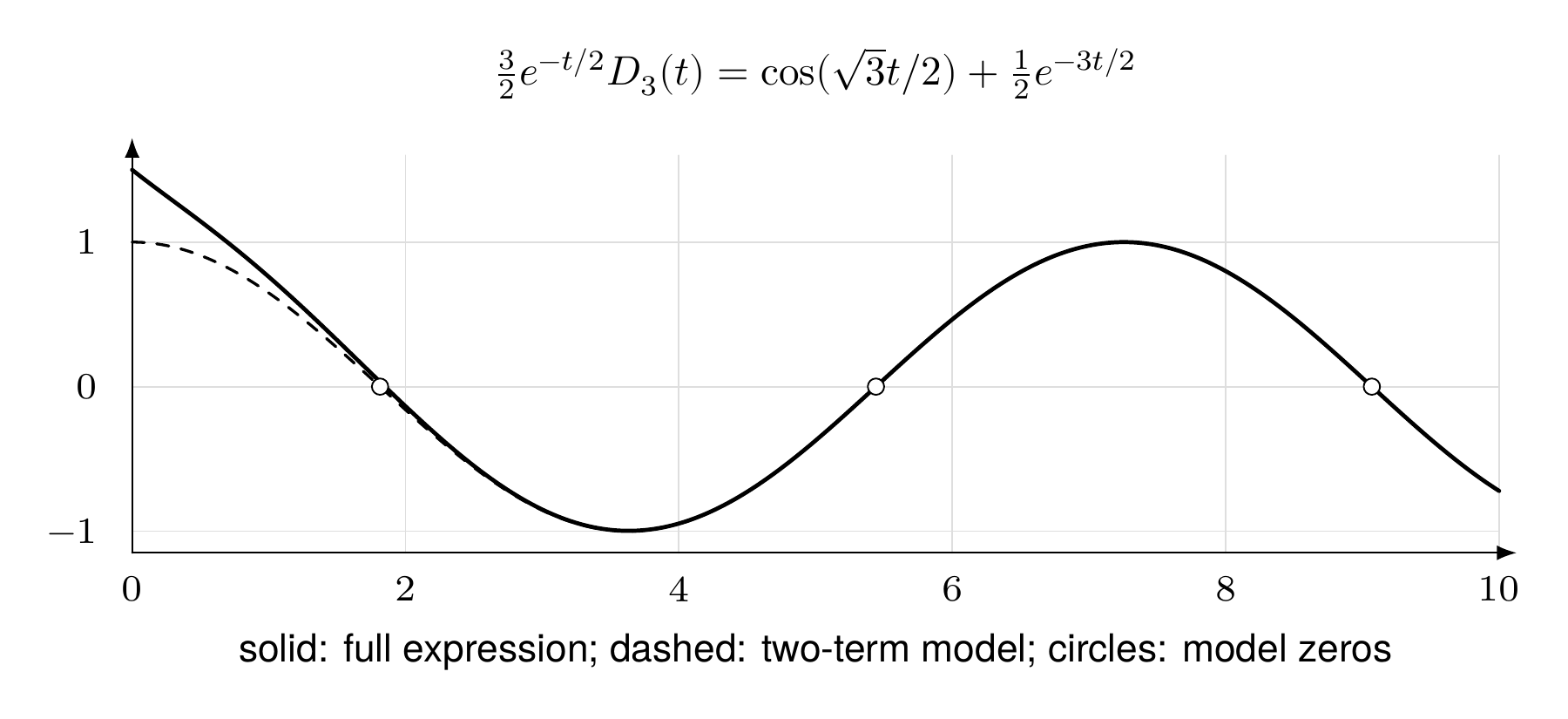
Reading the drawing
The horizontal axis is the real argument. The solid curve includes the small positive exponential remainder; the dashed curve omits it. Circles mark zeros of the cosine model. The solid crossings are slightly displaced from those markers, with displacement decreasing along the displayed positive direction. The next plate supplies separate rational certificates.
Drawing labels and data 11 labels
Read the original labels as selectable text. Tables preserve grid relationships; other short labels are grouped compactly.
Argument-axis ticks
\(0\), \(2\), \(4\), \(6\), \(8\), \(10\)
Value-axis ticks
\(-1\), \(0\), \(1\)
Normalized expression
Curve and marker key
solid: full expression; dashed: two-term model; circles: model zeros
Ignoring the last term gives model zeros
At \(t_m\), the full normalized expression equals \(\tfrac12e^{-3t_m/2}>0\), so \(t_m\) is not an exact zero. Linearizing the cosine at that point predicts
The alternating slope explains why the true zero is to the right of the first model zero, then to the left of the second, and so on in the eventual regime.
Symmetry needs uniqueness
Real coefficients alone allow nonreal conjugate pairs. The manuscript first proves that a near-model disk contains exactly one zero. Conjugation preserves that disk, so the unique zero must equal its conjugate. This additional uniqueness step, not the symmetry alone, places it exactly on the ray.
Read this as
The correction is caused by a real, nonzero remainder. A good cosine approximation does not make its model zeros exact.
Evidence note from the source edition
The curves are sampled analytic expressions. The next page independently certifies four narrow real-zero intervals rather than trusting the plotted crossing or the floating-point root finder.