
Take \(R=k[t]\) and the perfect complex
Specialization at \(t=a\) gives \(C_a=[k\xrightarrow{a}k]\). When \(a\ne0\), the differential is invertible and the complex is acyclic. When \(a=0\), the differential is zero and both cohomology groups survive.
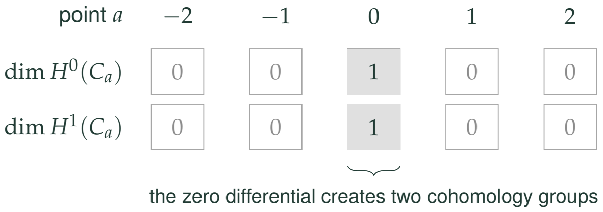
Reading the drawing
Five columns correspond to a equal to minus two, minus one, zero, one and two. The rows give dimensions of H zero and H one. Both dimensions are one at zero and zero at the other displayed points.
Drawing labels and data 19 labels
Read the original labels as selectable text. Tables preserve grid relationships; other short labels are grouped compactly.
- point \(a\)
- \(\dim H^0(C_a)\)
- \(\dim H^1(C_a)\)
- \(-2\)
- \(-1\)
- \(0\)
- \(1\)
- \(2\)
- \(0\)
- \(0\)
- \(0\)
- \(0\)
- \(0\)
- \(0\)
- \(0\)
- \(0\)
- \(1\)
- \(1\)
the zero differential creates two cohomology groups
Evidence note from the source edition
A few fibers over \(k={\mathbb Q}\) are displayed. The statement for every \(a\ne0\) follows from invertibility of the scalar \(a\); it is not inferred from the sample points.
Compute before and after specialization
Before specialization,
After derived specialization at zero,
If one retained only \(H^1(C)\) and took its ordinary tensor product with \(k\), one would see a single \(k\) and miss the extra cohomology in degree zero. The projective complex keeps the information needed for specialization.
The support is still a precise locus
At any prime not containing \(t\), the residue-field differential is invertible. At the prime \((t)\) it is zero. Therefore
Theorem 6.16 identifies support after derived quotient with the intersection of original support and the quotient locus.
Read this as
Derived nonvanishing means that some cohomology group survives after derived specialization. It neither specifies a classical automorphic class nor eliminates the need for a realization theorem.