
Fix \({\mathcal O}={\mathbb Z}_5\). Take two independent local variables and impose two different kinds of condition:
Their completed local tensor is \(A={\mathcal O}[[x,y]]\). The closed generated ideal is \(J=(x^2,y)\), and both routes through Theorem 3.1 give
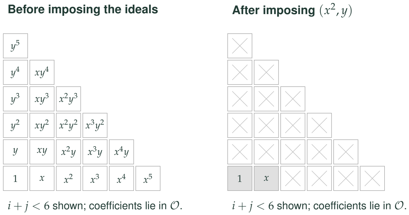
Reading the drawing
Two triangular windows show monomials of total degree below six. Before the quotient every displayed monomial is present. After imposing x squared and y, only one and x remain. Crosses mark monomials killed by the ideal; they are not small coefficients.
Drawing labels and data 27 labels
Read the original labels as selectable text. Tables preserve grid relationships; other short labels are grouped compactly.
- Before imposing the ideals
- \(1\)
- \(x\)
- \(x^{2}\)
- \(x^{3}\)
- \(x^{4}\)
- \(x^{5}\)
- \(y\)
- \(xy\)
- \(x^{2}y\)
- \(x^{3}y\)
- \(x^{4}y\)
- \(y^{2}\)
- \(xy^{2}\)
- \(x^{2}y^{2}\)
- \(x^{3}y^{2}\)
- \(y^{3}\)
- \(xy^{3}\)
- \(x^{2}y^{3}\)
- \(y^{4}\)
- \(xy^{4}\)
- \(y^{5}\)
\(i+j<6\) shown; coefficients lie in \(\mathcal O\).
- After imposing \((x^2,y)\)
- \(1\)
- \(x\)
\(i+j<6\) shown; coefficients lie in \(\mathcal O\).
Evidence note from the source edition
An exact finite window of monomials over \({\mathcal O}\). Crosses mean that the monomial is zero in the quotient; they do not represent a small numerical coefficient. All terms outside the window satisfy the same divisibility rule.
The calculation behind the image
For \(f=\sum_{i,j\ge0}a_{ij}x^iy^j\), reduction gives
Every term involving \(y\) vanishes. Every term involving \(x^2\) vanishes. The class of \(x\) does not vanish: it becomes a nonzero element whose square is zero. The quotient is a free \({\mathcal O}\)-module with basis \(1,\varepsilon\).
Why a point picture alone would miss this
After passing to the special fiber, \(k[\varepsilon]/(\varepsilon^2)\) has the same underlying one-point spectrum as \(k\). The extra direction is visible in the algebra and in maps from test rings, not as a second point. It is also not a second component or a second Artin packet.
Read this as
The condition \(y=0\) deletes a variable. The condition \(x^2=0\) retains a first-order nilpotent direction. Both are quotient conditions, but their effects are different.