
8 Packetwise mixed precision
On this page · Visual guide: The objects and their contracts · Permalink · Source line 1250
8.1 One operator
On this page · Permalink · Source line 1252
Theorem 8.1: Packet perturbation certificate
Let
where edge \(e\) starts at packet \(\alpha(e)\), and assume
Then
If
then
Read proof · Visual guide: Twelve small blocks, one coherent error · Read statement and proof side by side · Permalink · Source line 1254 · Claim record · Lean coverage · Code · Worked examples
Proof of Theorem 8.1
Exact packet evaluation gives
Apply the triangle inequality and the operator norm bound to each term.
Back to statement · Read statement and proof side by side · Permalink · Source line 1298 · Claim record · Lean coverage · Code · Worked examples
Standard fact 8.2: Floating point matrix product model
For real \(A\in{\mathbb R}^{m\times p}\) and \(B\in{\mathbb R}^{p\times n}\), consider ordinary dot-product matrix multiplication in uniform precision with unit roundoff \(u\), no overflow or underflow, and \(pu<1\). Its computed output \(\widehat C\) satisfies the componentwise forward-error bound
Absolute values and the inequality are entrywise. Complex arithmetic, fused kernels, mixed accumulation, and tensor kernels require their own stated constants. This fact does not assert one common small input perturbation for every column, and an input-dependent rounded action is not automatically a fixed linear operator.
Permalink · Source line 1308 · Claim record · Lean coverage · Code · Worked examples
Detailed forms and their hypotheses are given in [Higham2002], [HighamMary2021]. For a fixed computed matrix, the bound can certify its error matrix. A rounded application to varying inputs needs a separately justified uniform certificate before it can be used as one fixed operator error in Theorem 8.1.
8.2 Several operators
On this page · Permalink · Source line 1319
Corollary 8.3: Mixed precision product chain
If each fixed linear factor \(A_j\) is replaced by a fixed packetwise linear approximation \(\widehat A_j\), write \(E_j=\widehat A_j-A_j=\sum_e\Delta_{j,e}P_{\alpha(j,e)}\). A uniform certificate is
For orthogonal packet projectors, \(\delta_j\le\sum_e\|\Delta_{j,e}\|\). The final operator error is bounded by Theorem 5.8 with these uniform \(\delta_j\). The corresponding vector error is this operator bound multiplied by the input norm.
Read proof · Read statement and proof side by side · Permalink · Source line 1321 · Claim record · Lean coverage · Code · Worked examples
Proof of Corollary 8.3
Take the supremum over unit inputs in Theorem 8.1, using \(\|P_{\alpha}x\|\le\|P_{\alpha}\|\|x\|\). Substitute the resulting uniform operator error bounds into Theorem 5.8; the action estimate follows from submultiplicativity.
Back to statement · Read statement and proof side by side · Permalink · Source line 1329 · Claim record · Lean coverage · Code · Worked examples
8.3 Continuous allocation
On this page · Permalink · Source line 1333
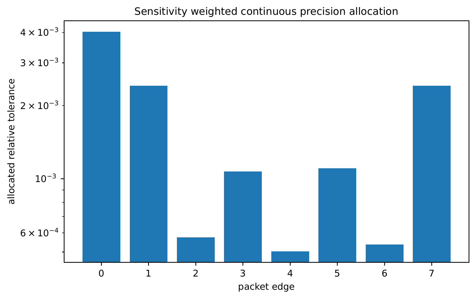
Theorem 8.4: Continuous precision allocation
Let \(E\) be a finite nonempty edge set, let \(s_e>0\) be sensitivities and \(c_e>0\) be costs, and let \(\tau>0\). Consider
subject to
The unique minimizer is
Read proof · Visual guide: Spend error where it is cheapest · Read statement and proof side by side · Permalink · Source line 1335 · Claim record · Lean coverage · Code · Worked examples
Proof of Theorem 8.4
The Lagrangian derivative gives
Thus
The constraint gives
The objective is strictly convex on the positive orthant, so the stationary point is the unique minimizer.
Back to statement · Read statement and proof side by side · Permalink · Source line 1355 · Claim record · Lean coverage · Code · Worked examples
Theorem 8.5: Clipped precision allocation
Retain the finite nonempty edge set, strictly positive sensitivities and costs, and add strictly positive caps \(m_e>0\) with upper bounds
Assume
There is a unique \(\lambda>0\), except at the maximal tolerance endpoint, such that
and
This vector minimizes the same objective over the clipped feasible set.
Read proof · Visual guide: Spend error where it is cheapest · Read statement and proof side by side · Permalink · Source line 1371 · Claim record · Lean coverage · Code · Worked examples
Proof of Theorem 8.5
The Karush Kuhn Tucker conditions give the unconstrained form on every nonactive coordinate and equality with \(m_e\) on every active upper bound. The weighted sum
is continuous and nonincreasing. It decreases from the maximal feasible value to zero. For a strictly submaximal budget, once any coordinate is unsaturated, \(\phi\) is strictly decreasing, which gives a unique multiplier. At maximal budget the only feasible vector is \((m_e)_e\) and every \(0<\lambda\le\min_e c_e/(s_em_e)\) produces it. Thus the minimizing vector is unique at this endpoint while its multiplier need not be. Strict convexity gives uniqueness of the minimizer in every case.
Back to statement · Read statement and proof side by side · Permalink · Source line 1398 · Claim record · Lean coverage · Code · Worked examples
8.4 Discrete data types
On this page · Permalink · Source line 1419
Definition 8.6: Discrete precision option
For edge \(e\), a discrete precision option \(k\) has a measured or modeled cost \(c_{e,k}\) and a nonnegative integer error weight \(w_{e,k}\). Exactly one option must be selected on every edge.
Permalink · Source line 1421 · Claim record · Lean coverage · Code · Worked examples
Theorem 8.7: Exact discrete precision program
Let the total integer error budget be \(B\). Define
as the minimum cost for assigning precisions to the first \(j\) edges with total weight exactly \(b\). Then
Set \(F_{j-1}(u)=+\infty\) whenever \(u<0\) or the state is unreachable. Then
The minimum of \(F_m(b)\) over \(0\leq b\leq B\) is the exact minimum cost for the quantized model.
Read proof · Visual guide: An exact budget is not a greedy choice · Visual guide: Safe integers can still be conservative · Read statement and proof side by side · Permalink · Source line 1425 · Claim record · Lean coverage · Code · Worked examples
Proof of Theorem 8.7
Every feasible assignment for the first \(j\) edges ends with one option \(k\) on edge \(j\). Removing it leaves an optimal or suboptimal assignment for the first \(j-1\) edges with residual weight \(b-w_{j,k}\). Replacing a suboptimal prefix by an optimal one can only lower cost. The recurrence therefore has optimal substructure. Induction on \(j\) proves the result.
Back to statement · Read statement and proof side by side · Permalink · Source line 1451 · Claim record · Lean coverage · Code · Worked examples
Remark 8.8
The discrete program is exact only for the supplied options and quantized error weights. Real kernels also depend on accumulation type, scaling, overflow, underflow, tensor core availability, and shape restrictions. Mixed precision iterative refinement has its own conditioning requirements [CarsonHigham2018].
Visual guide: An exact budget is not a greedy choice · Permalink · Source line 1455