
E9 Bayesian coarsening and finite sufficiency
On this page · Permalink · Source line 3458
A fixed coarse description will be called sufficient when it reproduces the coarse posterior masses for every positive prior and leaves the conditional distribution inside every packet unchanged. This excludes a coarse rule that hides an unrecorded local update.
Let \(C\) send a fine probability vector to its block masses
Assume first that every block mass is positive. Write
for the prior conditional distribution inside packet \(I_\alpha\). Define the prior dependent packet average likelihood
Theorem E9.1: Exact two stage Bayesian update
For every strictly positive prior,
For every packet with \(\overline\lambda_\alpha(p)>0\), the posterior conditional distribution is
A packet with zero average likelihood has zero posterior mass. Thus a fine Bayesian update consists of a coarse update by packet average likelihoods followed by independent local updates inside the packets that survive.
Read proof · Read statement and proof side by side · Permalink · Source line 3481 · Claim record · Lean coverage · Code · Worked examples
Proof of Theorem E9.1
The posterior mass of packet \(I_\alpha\) is
This is the coarse Bayesian formula. Dividing the fine posterior coordinates by the packet mass gives the local formula.
Back to statement · Read statement and proof side by side · Permalink · Source line 3498 · Claim record · Lean coverage · Code · Worked examples
Theorem E9.2: Characterization of fixed coarse sufficiency
Assume \(\lambda_i>0\) for every state. The following conditions are equivalent.
There is a positive coarse likelihood \(\ell\in(0,\infty)^m\) such that
\[ C{\mathcal B}_\lambda(p) = {\mathcal B}_\ell(Cp) \]for every strictly positive prior \(p\), and the posterior conditional distribution inside every packet equals its prior conditional distribution.
The likelihood is constant on every packet.
When these conditions hold, \(\ell_\alpha\) can be chosen as the common value of \(\lambda\) on \(I_\alpha\), and it is unique up to a common positive scale.
Read proof · Read statement and proof side by side · Permalink · Source line 3510 · Claim record · Lean coverage · Code · Worked examples
Proof of Theorem E9.2
If \(\lambda\) is constant on each packet, Theorem E9.1 has packet averages independent of the prior and its local posterior formula gives \(q_\alpha=r_\alpha\). This proves the first condition.
Conversely, fix any strictly positive prior. Equality of the local posterior and prior conditionals gives
for every \(i\in I_\alpha\). Positivity of the conditional prior implies
for every state in the packet. Thus the likelihood is constant on every packet. If two positive coarse likelihoods define the same update for every positive coarse prior, comparison of any two posterior odds shows that their coordinate ratios agree. Hence they differ only by a common positive factor.
Back to statement · Read statement and proof side by side · Permalink · Source line 3525 · Claim record · Lean coverage · Code · Worked examples
Theorem E9.3: Coarsest fixed sufficient partition
Let \(\mathcal L\) be a nonempty family of strictly positive likelihood vectors. Define
Let \(\mathcal Q_{\mathcal L}\) be the partition into equivalence classes. A partition \(\mathcal Q\) gives a fixed coarse sufficient description in the sense of Theorem E9.2 for every \(\lambda\in\mathcal L\) if and only if every block of \(\mathcal Q\) is contained in a block of \(\mathcal Q_{\mathcal L}\). Hence \(\mathcal Q_{\mathcal L}\) is the unique coarsest partition with this property.
Read proof · Visual guide: Several observations determine one sufficient partition · Read statement and proof side by side · Permalink · Source line 3542 · Claim record · Lean coverage · Code · Worked examples
Proof of Theorem E9.3
Apply Theorem E9.2 to every likelihood in the family. A fixed sufficient description exists exactly when each likelihood is constant on every block of \(\mathcal Q\). This is equivalent to every block of \(\mathcal Q\) being contained in one common level set of the family. The equivalence class partition is itself admissible, and every other admissible partition refines it.
Back to statement · Read statement and proof side by side · Permalink · Source line 3553 · Claim record · Lean coverage · Code · Worked examples
Definition E9.4: Within packet information loss
For a prior \(p\), define
Then
Permalink · Source line 3557 · Claim record · Lean coverage · Code · Worked examples
Proposition E9.5: Exact local distortion
For every packet with positive mass and evidence,
Consequently,
If \(\lambda\) is positive on the packet, then
Read proof · Read statement and proof side by side · Permalink · Source line 3571 · Claim record · Lean coverage · Code · Worked examples
Proof of Proposition E9.5
Subtract \(r_{\alpha,i}\) from the local posterior formula in Theorem E9.1. The norm identity follows because the factor multiplying \(\eta_i\) is nonnegative. The last estimate uses
and \(\overline\lambda_\alpha(p)\geq\min_{I_\alpha}\lambda\).
Back to statement · Read statement and proof side by side · Permalink · Source line 3596 · Claim record · Lean coverage · Code · Worked examples
Theorem E9.6: Approximate coarse Bayesian rule
Choose one positive number \(\ell_\alpha\) for every packet and define the block constant fine likelihood
Then
Read proof · Read statement and proof side by side · Permalink · Source line 3606 · Claim record · Lean coverage · Code · Worked examples
Proof of Theorem E9.6
Block constancy gives
Aggregation is an \(\ell^1\) contraction. Apply Theorem E8.3 to the two fine posteriors and then aggregate.
Back to statement · Read statement and proof side by side · Permalink · Source line 3626 · Claim record · Lean coverage · Code · Worked examples
Definition E9.7: Relative information
For probability vectors \(q\) and \(p\), define
The convention is \(0\log0=0\). A term with \(q_i>0\) and \(p_i=0\) has value \(+\infty\).
Permalink · Source line 3636 · Claim record · Lean coverage · Code · Worked examples
Theorem E9.8: Exact information decomposition
Let \(p\) and \(q\) be probability vectors on a finite partition \((I_\alpha)_\alpha\), and assume \(q_i=0\) whenever \(p_i=0\). Let
and let \(p_\alpha\) and \(q_\alpha\) be the conditional distributions inside packet \(I_\alpha\) whenever the corresponding mass is positive. Then
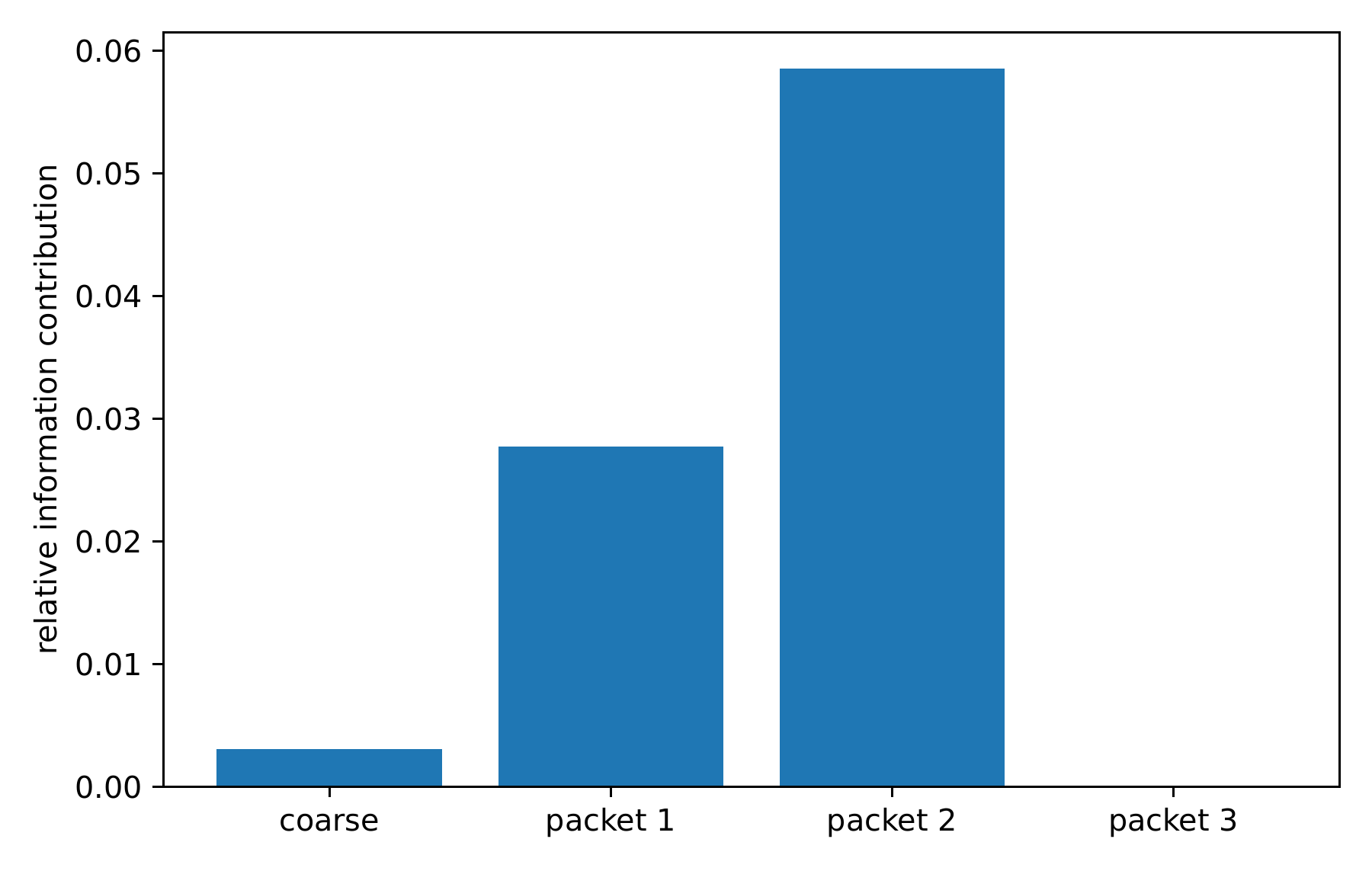
The first term is the information retained by the coarse masses. The second term is the exact information carried by changes inside the packets.
Read proof · Visual guide: Information loss has an exact location · Read statement and proof side by side · Permalink · Source line 3646 · Claim record · Lean coverage · Code · Worked examples
Proof of Theorem E9.8
For \(i\in I_\alpha\), write
Then
Multiply by \(q_i\), sum first inside each packet, and then sum over the packets. This is the finite relative entropy chain rule. Standard information theoretic treatments include [CoverThomas2006].
Back to statement · Read statement and proof side by side · Permalink · Source line 3665 · Claim record · Lean coverage · Code · Worked examples
Corollary E9.9: Coarse data processing and equality
Under the assumptions of Theorem E9.8,
Equality holds if and only if
for every packet with positive posterior mass.
Read proof · Visual guide: Information loss has an exact location · Read statement and proof side by side · Permalink · Source line 3683 · Claim record · Lean coverage · Code · Worked examples
Proof of Corollary E9.9
Every conditional relative information term in Theorem E9.8 is nonnegative. It vanishes exactly when the two conditional distributions agree.
Back to statement · Read statement and proof side by side · Permalink · Source line 3697 · Claim record · Lean coverage · Code · Worked examples
Corollary E9.10: Information created by a Bayesian update
Let \(q={\mathcal B}_\lambda(p)\) with positive likelihood and positive prior. Then
Inside a packet,
Hence
Read proof · Read statement and proof side by side · Permalink · Source line 3701 · Claim record · Lean coverage · Code · Worked examples
Proof of Corollary E9.10
The posterior ratio is
The local ratio is
Insert these identities into the definition of relative entropy. The final estimate follows because both \(\lambda_i\) and the packet average lie between the packet minimum and maximum.
Back to statement · Read statement and proof side by side · Permalink · Source line 3728 · Claim record · Lean coverage · Code · Worked examples
Corollary E9.11: Information criterion for local sufficiency
For a fixed positive likelihood, the within packet term in Theorem E9.8 vanishes for every positive prior if and only if the likelihood is constant on every packet.
Read proof · Read statement and proof side by side · Permalink · Source line 3744 · Claim record · Lean coverage · Code · Worked examples
Proof of Corollary E9.11
If the likelihood is block constant, every local posterior equals its local prior. Conversely, choose any positive prior. Vanishing relative entropy gives \(q_\alpha=r_\alpha\). The local posterior formula then forces all likelihood values in that packet to equal their packet average. Repeat for every packet.
Back to statement · Read statement and proof side by side · Permalink · Source line 3748 · Claim record · Lean coverage · Code · Worked examples
Remark E9.12
The exact coarse likelihood in Theorem E9.1 depends on the conditional prior inside each packet. Theorem E9.2 identifies when that dependence disappears. Theorem E9.8 measures what is lost when only the coarse posterior masses are retained.