Paper VI: Green operators and finite difference transfer

E12 Green operators and finite difference transfer

On this page · Permalink · Source line 4138

Consider

\[ -u''=f \quad\hbox{on }(0,1), \qquad u(0)=u(1)=0. \]

The continuum Green kernel is

\[ G(x,y)=\min(x,y)-xy. \]

Thus

\[ u(x)=\int_0^1G(x,y)f(y){\,\mathrm d} y. \]

For \(n\) interior nodes, let

\[ h=\frac{1}{n+1}, \qquad x_i=ih, \]

and define

\[ L_h = \frac{1}{h^2} \begin{pmatrix} 2&-1&&\\ -1&2&\ddots&\\ &\ddots&\ddots&-1\\ &&-1&2 \end{pmatrix}. \]

Permalink · Source line 4140

Theorem E12.1: Exact nodal Green reconstruction

For \(1\leq i,j\leq n\),

\[ \frac{1}{h}(L_h^{-1})_{ij} = G(x_i,x_j). \]

Read proof · Read statement and proof side by side · Permalink · Source line 4175 · Claim record · Lean coverage · Code · Worked examples

Proof of Theorem E12.1

The inverse of the unscaled tridiagonal matrix has entry

\[ \frac{\min(i,j)(n+1-\max(i,j))}{n+1}. \]

Multiplying by \(h^2\) and dividing by \(h\) gives

\[ h\min(i,j) \left(1-\frac{\max(i,j)}{n+1}\right) = \min(x_i,x_j)-x_ix_j. \]

Back to statement · Read statement and proof side by side · Permalink · Source line 4184 · Claim record · Lean coverage · Code · Worked examples

Corollary E12.2: Discrete Green quadrature

If \(u^h\) solves

\[ L_hu^h=f^h, \]

then every nodal value has the exact representation

\[ u_i^h = h\sum_{j=1}^nG(x_i,x_j)f_j^h. \]

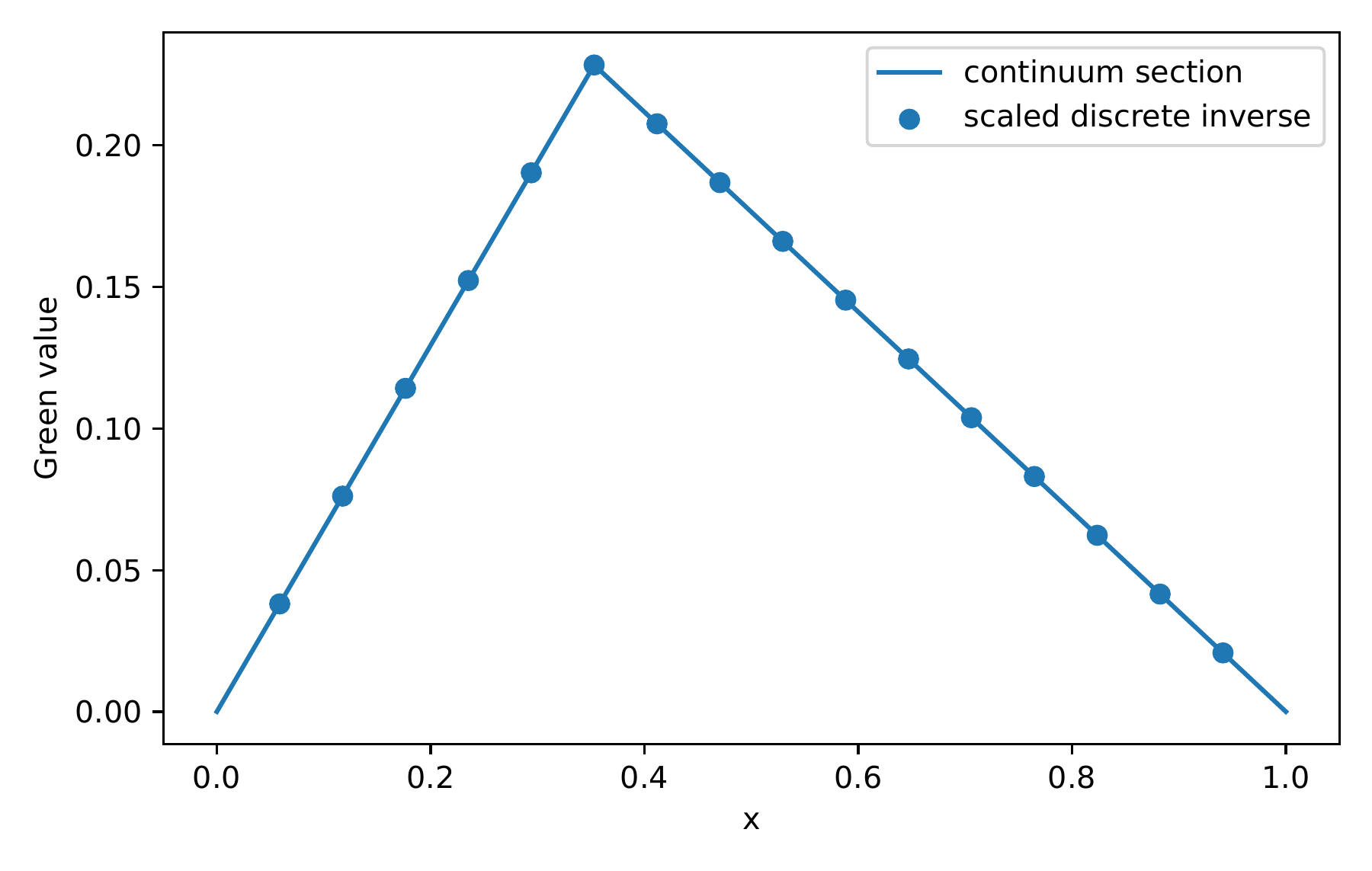
Thus the discrete Green operator is the nodal rectangle quadrature of the continuum Green kernel.

Read proof · Read statement and proof side by side · Permalink · Source line 4198 · Claim record · Lean coverage · Code · Worked examples

Proof of Corollary E12.2

By Theorem E12.1,

\[ (L_h^{-1})_{ij}=hG(x_i,x_j). \]

Multiply the inverse matrix by the source vector.

Back to statement · Read statement and proof side by side · Permalink · Source line 4212 · Claim record · Lean coverage · Code · Worked examples

Proposition E12.3: Discrete maximum bound

The inverse \(L_h^{-1}\) has nonnegative entries and

\[ {\left\lVert L_h^{-1}\right\rVert}_{\infty\to\infty} = \max_{1\leq i\leq n} \frac{x_i(1-x_i)}{2} \leq \frac18. \]

Read proof · Read statement and proof side by side · Permalink · Source line 4220 · Claim record · Lean coverage · Code · Worked examples

Proof of Proposition E12.3

Nonnegativity follows from the entry formula in Theorem E12.1. Let \(v_i=x_i(1-x_i)/2\). Since the second difference is exact on quadratics,

\[ L_hv={{\boldsymbol{1}}}. \]

Hence the \(i\)th row sum of \(L_h^{-1}\) is \(v_i\). For a nonnegative matrix, the infinity operator norm is the largest row sum.

Back to statement · Read statement and proof side by side · Permalink · Source line 4232 · Claim record · Lean coverage · Code · Worked examples

Theorem E12.4: Second order Poisson solution error

Suppose \(u\in C^4[0,1]\) solves the Dirichlet problem above. Let

\[ f^h_i=f(x_i) \]

and let \(u^h\) solve

\[ L_hu^h=f^h. \]

Then

\[ \max_i{\left\lvert u^h_i-u(x_i)\right\rvert} \leq \frac{h^2}{96} {\left\lVert u^{(4)}\right\rVert}_\infty. \]

Read proof · Read statement and proof side by side · Permalink · Source line 4240 · Claim record · Lean coverage · Code · Worked examples

Proof of Theorem E12.4

Taylor expansion with remainder gives

\[ {\left\lVert L_h(u(x_i))_i-f^h\right\rVert}_\infty \leq \frac{h^2}{12}{\left\lVert u^{(4)}\right\rVert}_\infty. \]

Apply \(L_h^{-1}\) and use Proposition E12.3.

Back to statement · Read statement and proof side by side · Permalink · Source line 4258 · Claim record · Lean coverage · Code · Worked examples

The continuum Dirichlet Green section and the scaled discrete inverse. The nodal values agree exactly.

The discrete eigenpairs are

\[ \lambda_{k,h} = \frac{4}{h^2} \sin^2\left(\frac{k\pi h}{2}\right), \qquad v_{k,h}(i)=\sin(k\pi x_i). \]

Permalink · Source line 4275

Theorem E12.5: Low mode eigenvalue control

For \(kh\leq1\),

\[ 0\leq(k\pi)^2-\lambda_{k,h} \leq \frac{(k\pi)^4}{12}h^2. \]

Consequently, for every fixed \(k\),

\[ \lambda_{k,h}=(k\pi)^2+O(h^2). \]

Read proof · Read statement and proof side by side · Permalink · Source line 4285 · Claim record · Lean coverage · Code · Worked examples

Proof of Theorem E12.5

Set \(x=k\pi h/2\). The condition \(kh\leq1\) gives \(0\leq x\leq\pi/2\). On this interval,

\[ \sin x\geq x-\frac{x^3}{6}, \]

\[ 0\leq x^2-\sin^2x\leq\frac{x^4}{3}. \]

Multiply by \(4/h^2\).

Back to statement · Read statement and proof side by side · Permalink · Source line 4298 · Claim record · Lean coverage · Code · Worked examples

Corollary E12.6: Heat and fractional mode transfer

Let \(\lambda_k=(k\pi)^2\). For \(t\geq0\),

\[ 0\leq {\mathrm e}^{-t\lambda_{k,h}}-{\mathrm e}^{-t\lambda_k} \leq \frac{t(k\pi)^4}{12}h^2{\mathrm e}^{-t\lambda_{k,h}}. \]

For \(0<\alpha\leq1\) and fixed \(k\),

\[ \lambda_{k,h}^\alpha = \lambda_k^\alpha+O(h^2) \]

and

\[ {\mathrm e}^{-t\lambda_{k,h}^\alpha} = {\mathrm e}^{-t\lambda_k^\alpha}+O(th^2) \]

uniformly for \(t\) in bounded intervals.

Read proof · Read statement and proof side by side · Permalink · Source line 4310 · Claim record · Lean coverage · Code · Worked examples

Proof of Corollary E12.6

The ordinary heat estimate follows from the mean value theorem and Theorem E12.5. For fixed \(k\), the eigenvalues stay uniformly away from zero once \(h\) is small. The function \(x^\alpha\) is then Lipschitz on a common compact interval containing both eigenvalues. Apply the mean value theorem twice.

Back to statement · Read statement and proof side by side · Permalink · Source line 4333 · Claim record · Lean coverage · Code · Worked examples

Finite difference schemes and their stability theory are treated more broadly in [Strikwerda2004]. The present result uses the special one dimensional Green structure to obtain an explicit constant.

Permalink · Source line 4337

Read and explore

Proofs and implementation

About this work

Other resources