Paper VI: Bayesian flows and hidden Markov recursion

E10 Bayesian flows and hidden Markov recursion

On this page · Permalink · Source line 3764

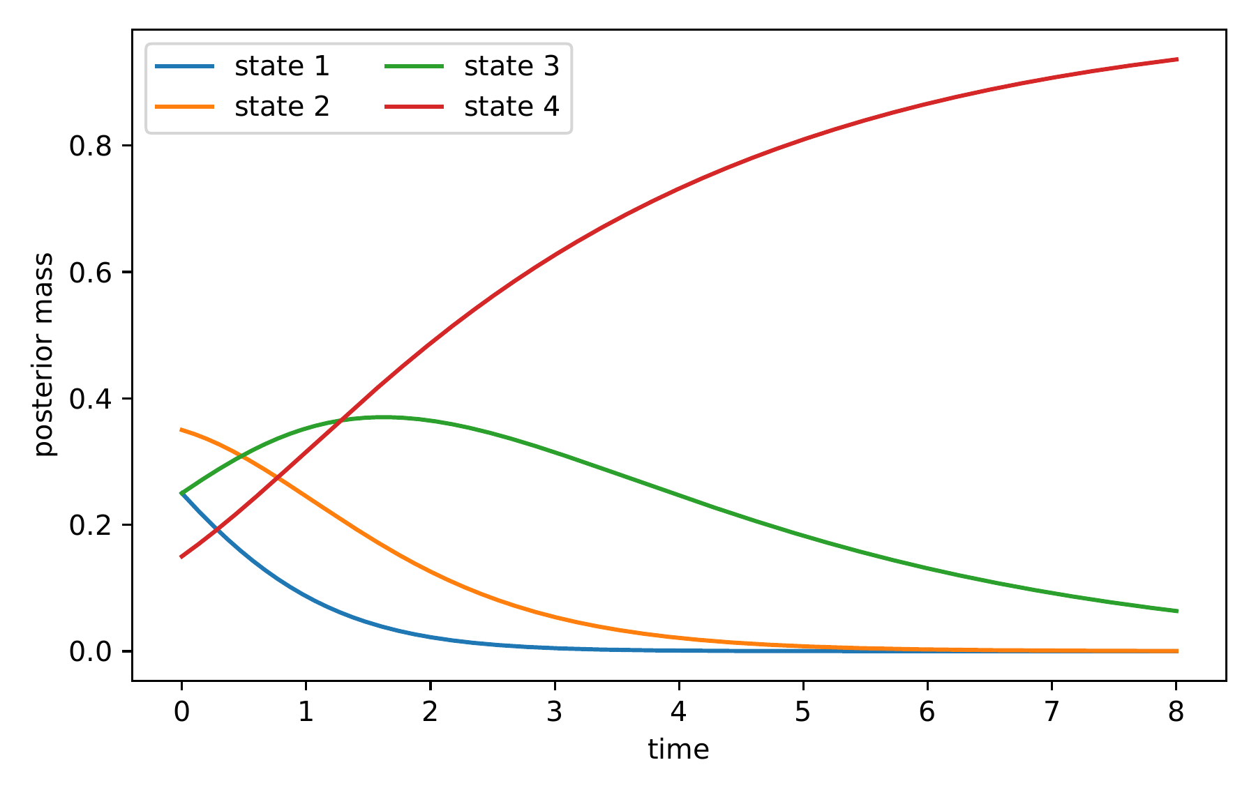
Fix a score vector \(g\in{\mathbb R}^n\). For \(t\geq0\), define

\[ \Phi_t(p)_i = \frac{{\mathrm e}^{tg_i}p_i} {\sum_j{\mathrm e}^{tg_j}p_j}. \]

Permalink · Source line 3766

Theorem E10.1: Bayesian flow and replicator equation

The maps \(\Phi_t\) form a nonlinear semigroup:

\[ \Phi_{s+t}=\Phi_s\circ\Phi_t. \]

Every coordinate satisfies

\[ \frac{{\,\mathrm d}}{{\,\mathrm d} t}p_i(t) = \bigl(g_i-{\left\langle g,p(t)\right\rangle}\bigr)p_i(t). \]

The support of \(p(t)\) is independent of \(t\), and for any two coordinates in the support,

\[ \frac{p_i(t)}{p_j(t)} = {\mathrm e}^{t(g_i-g_j)} \frac{p_i(0)}{p_j(0)}. \]

Read proof · Visual guide: The score rises because it has variance · Read statement and proof side by side · Permalink · Source line 3774 · Claim record · Lean coverage · Code · Worked examples

Proof of Theorem E10.1

The semigroup law follows from multiplication of the likelihoods \({\mathrm e}^{sg}\) and \({\mathrm e}^{tg}\). Differentiating the normalized formula gives the replicator equation. A coordinate that starts at zero remains zero, while a positive coordinate remains positive. Dividing two explicit coordinate formulas gives the odds identity.

Back to statement · Read statement and proof side by side · Permalink · Source line 3794 · Claim record · Lean coverage · Code · Worked examples

Theorem E10.2: Evidence cumulants and score monotonicity

Set

\[ \psi(t) = \log\left( \sum_i{\mathrm e}^{tg_i}p_i(0) \right). \]

Then

\[ \psi'(t)={\left\langle g,p(t)\right\rangle}, \qquad \psi''(t)={\operatorname{Var}}_{p(t)}(g)\geq0. \]

Consequently,

\[ \frac{{\,\mathrm d}}{{\,\mathrm d} t}{\left\langle g,p(t)\right\rangle} = {\operatorname{Var}}_{p(t)}(g). \]

Read proof · Visual guide: The score rises because it has variance · Read statement and proof side by side · Permalink · Source line 3798 · Claim record · Lean coverage · Code · Worked examples

Proof of Theorem E10.2

Differentiate the log normalizing constant once and twice. The second derivative is the centered second moment under the tilted distribution.

Back to statement · Read statement and proof side by side · Permalink · Source line 3821 · Claim record · Lean coverage · Code · Worked examples

Corollary E10.3: Concentration on the maximal score packet

Let

\[ G=\max\{g_i:p_i(0)>0\} \]

and let \(M\) be the set of supported indices with score \(G\). If \(M\) is the full support, then the conclusion below is immediate. Otherwise, suppose

\[ \delta = \min\{G-g_i:p_i(0)>0, \quad i\notin M\}>0. \]

Then

\[ 1-\sum_{i\in M}p_i(t) \leq \frac{1-p_M(0)}{p_M(0)}{\mathrm e}^{-\delta t}, \]

where \(p_M(0)=\sum_{i\in M}p_i(0)\).

Read proof · Read statement and proof side by side · Permalink · Source line 3825 · Claim record · Lean coverage · Code · Worked examples

Proof of Corollary E10.3

Factor \({\mathrm e}^{tG}\) from the normalizing constant. The total weight outside \(M\) is at most \((1-p_M(0)){\mathrm e}^{-\delta t}\), while the weight on \(M\) is \(p_M(0)\).

Back to statement · Read statement and proof side by side · Permalink · Source line 3846 · Claim record · Lean coverage · Code · Worked examples

A finite Bayesian flow. Mass concentrates on the states with the largest score, while every relative odds ratio follows an exact exponential law.

E10.1 Prediction and update

On this page · Permalink · Source line 3857

Let \(K\) be column stochastic and let \(\lambda^{(r)}\) be the likelihood of the \(r\)th observation. The hidden Markov filter is

\[ \widehat p_r=Kp_{r-1}, \qquad p_r={\mathcal B}_{\lambda^{(r)}}(\widehat p_r). \]

A standard account of finite hidden Markov models appears in [Rabiner1989].

Permalink · Source line 3859

Proposition E10.4: Simplex preservation

Suppose \(p_{r-1}\) is a probability vector and the new evidence is positive. Prediction produces the probability vector \(\widehat p_r\), and normalization produces the probability vector \(p_r\).

Read proof · Read statement and proof side by side · Permalink · Source line 3867 · Claim record · Lean coverage · Code · Worked examples

Proof of Proposition E10.4

Column stochasticity preserves nonnegativity and total mass. Bayesian normalization then preserves the same properties.

Back to statement · Read statement and proof side by side · Permalink · Source line 3871 · Claim record · Lean coverage · Code · Worked examples

Theorem E10.5: One step filter stability

Let \(K\) and \(\widetilde K\) be column stochastic. Assume

\[ 0<a\leq\lambda_i\leq b. \]

Then

\[ {\left\lVert {\mathcal B}_\lambda(Kp)-{\mathcal B}_\lambda(\widetilde Kq) \right\rVert}_1 \leq \frac{2b}{a} \left( {\left\lVert p-q\right\rVert}_1 + {\left\lVert K-\widetilde K\right\rVert}_{1\to1} \right). \]

Read proof · Read statement and proof side by side · Permalink · Source line 3875 · Claim record · Lean coverage · Code · Worked examples

Proof of Theorem E10.5

Apply Theorem E8.4 to \(Kp\) and \(\widetilde Kq\). Then use

\[ {\left\lVert Kp-\widetilde Kq\right\rVert}_1 \leq {\left\lVert K(p-q)\right\rVert}_1 + {\left\lVert(K-\widetilde K)q\right\rVert}_1 \]

and the stochastic contraction property.

Back to statement · Read statement and proof side by side · Permalink · Source line 3895 · Claim record · Lean coverage · Code · Worked examples

Example E10.6: Beta binomial transfer

A beta prior with parameters \((a,b)\) and binomial data containing \(s\) successes in \(n\) trials gives the posterior parameters

\[ (a+s,b+n-s). \]

The update is additive in the two exponent coordinates. This is a finite dimensional conjugate realization of likelihood composition. Standard Bayesian references include [BernardoSmith1994].

Permalink · Source line 3907

Read and explore

Proofs and implementation

About this work

Other resources

E10 Bayesian flows and hidden Markov recursion

Theorem E10.1: Bayesian flow and replicator equation

Proof of Theorem E10.1

Theorem E10.2: Evidence cumulants and score monotonicity

Proof of Theorem E10.2

Corollary E10.3: Concentration on the maximal score packet

Proof of Corollary E10.3

E10.1 Prediction and update

Proposition E10.4: Simplex preservation

Proof of Proposition E10.4

Theorem E10.5: One step filter stability

Proof of Theorem E10.5

Example E10.6: Beta binomial transfer