
Take the unary operation \(f(x)=x^2\) over \({\mathbb Q}\). Suppose both input and output transport are chosen as multiplication by two, while the same numerical formula \(f\) is reused at the target. The two routes give
Their difference is \(-2x^2\), which is generally nonzero.
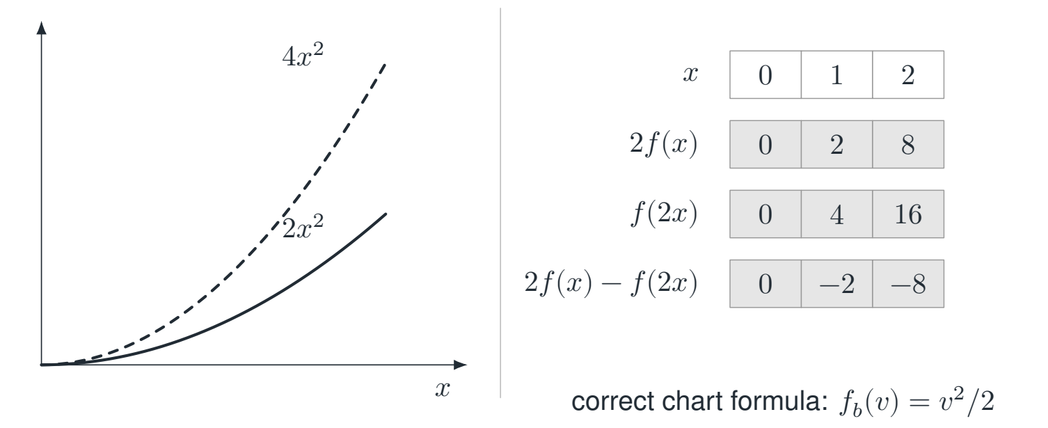
Reading the drawing
Solid and dashed parabolas display the two exact quadratic formulas. The table gives rational evaluations, showing the mismatch introduced by the chosen transport and rule.
Drawing labels and data 20 labels
Read the original labels as selectable text. Tables preserve grid relationships; other short labels are grouped compactly.
- \(2x^2\)
- \(4x^2\)
- \(x\)
| Row / column | Column 1 | Column 2 | Column 3 |
|---|---|---|---|
| \(x\) | \(0\) | \(1\) | \(2\) |
| \(2f(x)\) | \(0\) | \(2\) | \(8\) |
| \(f(2x)\) | \(0\) | \(4\) | \(16\) |
| \(2f(x)-f(2x)\) | \(0\) | \(-2\) | \(-8\) |
- correct chart formula: \(f_b(v)=v^2/2\)
Evidence note from the source edition
Solid: \(2x^2\). Dashed: \(4x^2\). The curves are a real visualization of exact polynomial formulas. The table contains exact evaluations over the rationals. The mismatch is caused by the specified combination of transport and formula.
For a canonical coordinate change with input and output chart \(v=2x\), the target formula is not still \(v^2\). It is
Consequently \(\widehat f_b(2x)=2x^2\), and the exact coordinate defect vanishes. This is the same distinction illustrated in the example in two dimensions on V10.
An example is not a general propagation theorem
The polynomial calculation here is exact and checked symbolically. It explains a chosen node defect, while the traditional paper develops composition identities, iterated defects, fixed point stability, and derivative defects under explicit hypotheses. Those broader ordinary proofs must be read on their own terms. This one example and the finite Lean locality theorem do not certify them.
Read this as
A nonzero nonlinear route difference must come from identifiable extra data: a changed transport, an approximation, a restricted model, or a reused formula that was not conjugated correctly.