
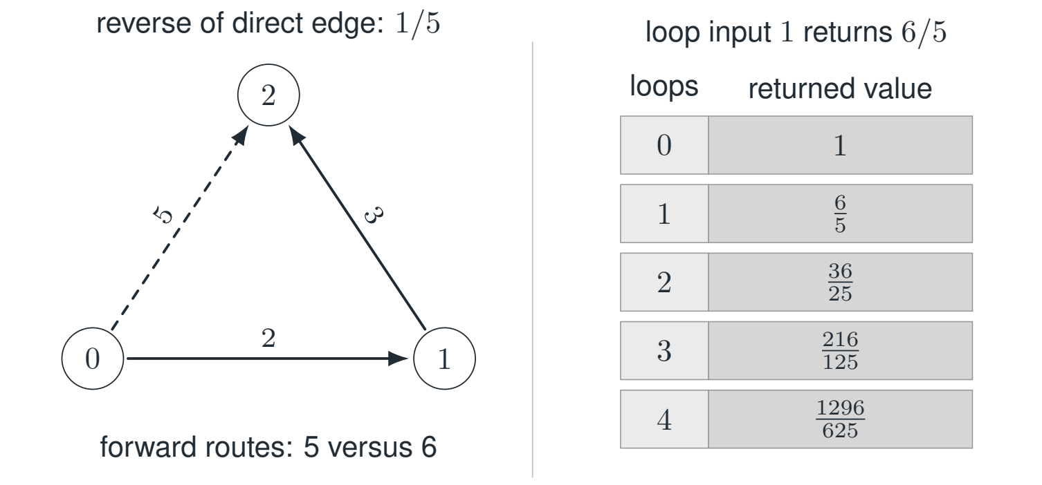
Retain the reversible scalar model with forward values \(2,3,5\) and all reverse values given by inverses. Two routes from chart \(0\) to chart \(2\) multiply the input by \(6\) and \(5\), respectively. The additive discrepancy equals the original input.
Reading the drawing
The dashed direct edge is a specified comparison map. The accompanying table records exact rational loop iterates rather than an analytic convergence assertion.
Drawing labels and data 21 labels
Read the original labels as selectable text. Tables preserve grid relationships; other short labels are grouped compactly.
- \(0\)
- \(1\)
- \(2\)
- \(2\)
- \(3\)
- \(5\)
- reverse of direct edge: \(1/5\)
- forward routes: 5 versus 6
- loop input \(1\) returns \(6/5\)
- \(0\)
- \(1\)
- \(1\)
\(\frac{6}{5}\)
- \(2\)
\(\frac{36}{25}\)
- \(3\)
\(\frac{216}{125}\)
- \(4\)
\(\frac{1296}{625}\)
- loops
- returned value
Evidence note from the source edition
The dashed direct edge is a specified comparison map, not a missing edge. The table shows the exact effect of traversing the same loop repeatedly. These are rational values of this example, not an analytic convergence claim.
The defect lives at the target of the forward routes:
The holonomy lives back at chart \(0\):
For input \(5\), the direct output and the output after two steps are \(25\) and \(30\). Returning by \(1/5\) gives \(5\) and \(6\). The target discrepancy of \(5\) has become a base discrepancy of \(1\). The types and locations of these differences matter even in an example in one dimension.
Because the return map is invertible, it cannot turn a nonzero defect into zero. This is the mechanism behind \(\Delta=0\Longleftrightarrow H=I\) in the reversible interface.
Read this as
Holonomy compares paths after both have been returned to the same base fiber. It is the transported mismatch, not an untyped difference between outputs in different charts.