Paper III: Nonlinear packet coordinates

Part II Nonlinear packet calculus, obstruction complexes, and holonomy

On this page · Permalink · Source line 1

This part moves from exact coordinates for arbitrary functions to differentiable interactions, specified correction problems, and finite or smooth transport. Each ordinary proof retains its stated hypotheses. These results are not asserted to belong to the finite Lean contract of Part I.

The notational change from \({\mathcal A},{\mathcal S}\) to \({\mathcal A},{\mathcal S}\) is typographical: both denote analysis and synthesis for the declared packet system. A connection remains additional data. Smooth canonical transport is constructed from a moving projector family, whereas the algebraic exact coordinate transport in Part I compares fixed exact descriptions of one ambient object.

Permalink · Source line 2

14 Introduction

On this page · Permalink · Source line 5

A finite family of pairwise annihilating idempotents gives exact coordinates. If

\[ P_\alpha P_\beta=0 \quad\text{for }\alpha\ne\beta, \qquad \sum_\alpha P_\alpha=I, \]

then every vector is the sum of its packet components. Linear operators become block matrices in these coordinates. A nonlinear map cannot be reconstructed from its diagonal restrictions, since mixed interactions between packet components are usually present. It can still be represented exactly if its input is the complete packet tuple.

This part develops nonlinear packet representation and the obstruction theory that follows from it. Exact coordinates preserve a nonlinear problem, but they do not solve it. Once the equation is written in packet coordinates, its derivatives, compositions, correction maps, refinement failures, and gluing defects can be separated without discarding mixed terms.

The first stage of Part II treats the local nonlinear calculus. Packet analysis and synthesis conjugate arbitrary maps. Fréchet derivatives split into multilinear packet jets. The higher chain rule then becomes a Faà di Bruno formula whose terms carry intermediate packet labels. Standard background on Fréchet calculus and the higher chain rule may be found in [AbrahamMarsdenRatiu1988], [ConstantineSavits1996], [Deimling1985].

The next stage studies nonlinear iteration. Repeated substitution is indexed by rooted trees rather than operator words. A scalar majorant gives an absolute convergence theorem for polynomial fixed point equations. The quadratic case recovers the Catalan series. Rooted tree combinatorics are discussed in [Stanley2012], [LodayVallette2012], [HairerLubichWanner2006].

A linear correction map

\[ D:U\longrightarrow V \]

places the obstruction to solving \(Du=-r\) in the canonical quotient \({\operatorname{coker}} D\). This quotient has a universal property and behaves naturally under commuting squares. Mapping cones extend the same construction to cochain complexes. In a Hilbert space with closed range, the quotient is represented by the orthogonal projection onto \({\operatorname{Ker}} D^*\). The Moore Penrose inverse then gives the least norm correction. Relevant background appears in [Weibel1994], [Penrose1955].

A vanishing linear obstruction is only the first step. We give a contraction theorem for nonlinear correction, followed by a local Lyapunov Schmidt reduction. In a complete filtered problem, every lifting step has its own cokernel class. Vanishing at all depths and compatible choices of corrections produce an exact inverse limit solution. A filtered correction complex carries a spectral sequence. Its first page records graded obstruction candidates, while later differentials record interactions that can cancel them. We use the standard spectral sequence of a filtered complex from [Weibel1994], [McCleary2001].

The final stage studies elimination and gluing. The implicit function theorem gives an exact Schur derivative after hidden variables are removed. Finite transport systems reduce, after a spanning tree gauge, to one holonomy element for each fundamental cycle. The same idea extends to smooth projector families through Kato transport. We use standard material from [Deimling1985], [GrossTucker1987], [Kato1950], [Kato1995], [KobayashiNomizu1963].

The article does not claim that every nonlinear problem has a finite obstruction space. The cokernel is canonical only after a correction map has been specified. It may be infinite dimensional. A first order obstruction may vanish while a higher order obstruction remains. The purpose of the calculus is to identify the exact object in which each failure lives and to show how those objects change under packets, refinement, filtration, and transport.

Permalink · Source line 7

15 A map of the nonlinear calculus

On this page · Permalink · Source line 35

Four questions organize the nonlinear calculus: representation, interaction, correction, and gluing.

The first question is representation. Given a nonlinear map \(F\), can its packet form be written without approximation? The answer is yes. Analysis and synthesis are inverse coordinate maps, so conjugation preserves the full equation.

The second question is interaction. Which input packets influence a given output packet, and at what derivative order? Packet jets answer this question. They form a directed hypergraph rather than an ordinary block matrix because one nonlinear interaction can have several inputs.

The third question is correction. Suppose an approximate solution leaves a defect \(r\). A declared linearized correction map \(D\) removes the part of \(r\) lying in \({\operatorname{im}} D\). The quotient class

\[ [r]\in{\operatorname{coker}} D \]

is the part that no allowed first order correction can remove. This quotient class is the obstruction. Its vanishing must be supplemented by a nonlinear theorem.

The fourth question is gluing. Local coordinate changes can solve every edge problem and still fail around a loop. The remaining cycle product is holonomy. It measures the failure of a global frame even when each local equation has been solved.

These four layers fit into the sequence

\[ \begin{gathered} \text{exact coordinates} \longrightarrow \text{packet interactions} \longrightarrow \text{correction classes} \\ \longrightarrow \text{global gluing}. \end{gathered} \]

Each arrow needs hypotheses. Exact coordinates need a complete packet system. Differential interactions need regularity. A cokernel obstruction needs a specified correction map. Holonomy needs invertible local transports.

A second distinction concerns scale. A refinement defect compares a fine nonlinear model with a coarse one. It is a point in the coarse output space. An obstruction class is the image of such a defect, or of another residual, in a quotient by allowed corrections. The correction map must be declared before the defect determines an obstruction class. A small defect can have a nonzero obstruction, and a large defect can have zero obstruction if it lies entirely in the correction range.

The paper uses finite packet systems in the coordinate and graph sections. Banach space hypotheses enter only where norms, contractions, or Fréchet derivatives are used. Module and complex language is used for cokernels, filtered lifting, and cohomological obstructions. This separation keeps each result at the level of generality supported by its proof.

Permalink · Source line 37

Standing conventions

On this page · Permalink · Source line 70

All packet systems are finite unless a statement says otherwise. In a normed setting every packet projector and every coarsening operator is bounded. Differentiability of operator valued maps is taken in operator norm. A Banach space isomorphism is a bounded linear bijection with bounded inverse. For a decreasing filtration \((F^mX)\), completeness means that the canonical map

\[ X\longrightarrow\varprojlim_m X/F^mX \]

is an isomorphism and separatedness means \(\bigcap_mF^mX=0\). Statements about congruence classes in a filtered nonlinear problem also assume that the nonlinear map preserves filtration congruences at the stated depth. These assumptions are repeated where they are essential to a proof.

Permalink · Source line 71

16 Exact nonlinear packet coordinates

On this page · Permalink · Source line 77

Let \(X\) be a module over a unital ring. A finite packet system on \(X\) is a family

\[ {\mathcal P}=(P_\alpha)_{\alpha\in I}\subseteq{\operatorname{End}}(X) \]

of nonzero idempotents such that

\[ P_\alpha P_\beta=0 \quad\text{when }\alpha\ne\beta, \qquad \sum_{\alpha\in I}P_\alpha=I_X. \]

Write

\[ X_\alpha=P_\alpha X, \qquad X^{{\mathcal P}}=\bigoplus_{\alpha\in I}X_\alpha. \]

The analysis and synthesis maps are

\[ {\mathcal A}_{{\mathcal P}}x=(P_\alpha x)_\alpha, \qquad {\mathcal S}_{{\mathcal P}}(x_\alpha)_\alpha=\sum_\alpha x_\alpha. \]

They are inverse isomorphisms.

Permalink · Source line 79

Definition 16.1: Nonlinear packet coordinate map

Let \({\mathcal P}\) be a packet system on \(X\) and let \({\mathcal Q}\) be a packet system on \(Y\). For any map \(F:X\to Y\), define

\[ F_{{\mathcal Q}\leftarrow{\mathcal P}} = {\mathcal A}_{{\mathcal Q}}F{\mathcal S}_{{\mathcal P}}. \]

Thus

\[ F_{{\mathcal Q}\leftarrow{\mathcal P}}((x_\alpha)_\alpha) = \left( Q_\gamma F\left(\sum_\alpha x_\alpha\right) \right)_\gamma. \]

Permalink · Source line 104 · Claim record · Lean coverage · Code · Worked examples

Theorem 16.2: Exact nonlinear coordinate theorem

For every map \(F:X\to Y\),

\[ {\mathcal S}_{{\mathcal Q}}F_{{\mathcal Q}\leftarrow{\mathcal P}}{\mathcal A}_{{\mathcal P}}=F. \]

If \(G:Y\to Z\) and \({\mathcal R}\) is a packet system on \(Z\), then

\[ (G\circ F)_{{\mathcal R}\leftarrow{\mathcal P}} = G_{{\mathcal R}\leftarrow{\mathcal Q}} \circ F_{{\mathcal Q}\leftarrow{\mathcal P}}. \]

No linearity, continuity, or differentiability assumption is needed.

Read proof · Read statement and proof side by side · Permalink · Source line 121 · Claim record · Lean coverage · Code · Worked examples

Proof of Theorem 16.2

The identities \({\mathcal S}_{{\mathcal P}}{\mathcal A}_{{\mathcal P}}=I_X\) and \({\mathcal S}_{{\mathcal Q}}{\mathcal A}_{{\mathcal Q}}=I_Y\) give

\[ {\mathcal S}_{{\mathcal Q}}F_{{\mathcal Q}\leftarrow{\mathcal P}}{\mathcal A}_{{\mathcal P}} = {\mathcal S}_{{\mathcal Q}}{\mathcal A}_{{\mathcal Q}}F{\mathcal S}_{{\mathcal P}}{\mathcal A}_{{\mathcal P}} =F. \]

For composition,

\[ G_{{\mathcal R}\leftarrow{\mathcal Q}}F_{{\mathcal Q}\leftarrow{\mathcal P}} = {\mathcal A}_{{\mathcal R}}G{\mathcal S}_{{\mathcal Q}}{\mathcal A}_{{\mathcal Q}}F{\mathcal S}_{{\mathcal P}} = {\mathcal A}_{{\mathcal R}}(G\circ F){\mathcal S}_{{\mathcal P}}. \]

Back to statement · Read statement and proof side by side · Permalink · Source line 137 · Claim record · Lean coverage · Code · Worked examples

Corollary 16.3: Dynamical equivalence

Suppose \(X=Y\) and the same packet system is used on both sides. Packet coordinates preserve fixed points, periodic points, injectivity, surjectivity, and invertibility. In particular,

\[ F(x)=x \quad\Longleftrightarrow\quad F_{{\mathcal P}\leftarrow{\mathcal P}}({\mathcal A}_{{\mathcal P}}x)={\mathcal A}_{{\mathcal P}}x. \]

Read proof · Read statement and proof side by side · Permalink · Source line 155 · Claim record · Lean coverage · Code · Worked examples

Proof of Corollary 16.3

The packet map is conjugate to \(F\) through the isomorphism \({\mathcal A}_{{\mathcal P}}\). Every listed property is invariant under conjugacy.

Back to statement · Read statement and proof side by side · Permalink · Source line 164 · Claim record · Lean coverage · Code · Worked examples

Proposition 16.4: Change of packet coordinates

Let \({\mathcal P}\) and \({\mathcal P}'\) be packet systems on \(X\). Let \({\mathcal Q}\) and \({\mathcal Q}'\) be packet systems on \(Y\). For any two packet systems \({\mathcal U}\) and \({\mathcal V}\) on the same space, write

\[ J_{{\mathcal U}\leftarrow{\mathcal V}} = {\mathcal A}_{{\mathcal U}}{\mathcal S}_{{\mathcal V}}. \]

Then

\[ F_{{\mathcal Q}'\leftarrow{\mathcal P}'} = J_{{\mathcal Q}'\leftarrow{\mathcal Q}} F_{{\mathcal Q}\leftarrow{\mathcal P}} J_{{\mathcal P}\leftarrow{\mathcal P}'}. \]

Read proof · Read statement and proof side by side · Permalink · Source line 168 · Claim record · Lean coverage · Code · Worked examples

Proof of Proposition 16.4

Insert \({\mathcal S}_{{\mathcal Q}}{\mathcal A}_{{\mathcal Q}}=I_Y\) and \({\mathcal S}_{{\mathcal P}}{\mathcal A}_{{\mathcal P}}=I_X\) into the definition of \(F_{{\mathcal Q}'\leftarrow{\mathcal P}'}\).

Back to statement · Read statement and proof side by side · Permalink · Source line 185 · Claim record · Lean coverage · Code · Worked examples

Exactness by cancellation

Analysis and synthesis undo each other on the complete packet tuple. In a composition of packet descriptions, the intermediate synthesis and analysis maps cancel. This compares exact descriptions of the same ambient object. A connection adds data for transport along parameters or paths, with its own hypotheses.

Permalink · Source line 189

Example 16.5: A mixed quadratic map

Let \(X=Y={\Bbbk}^2\) with coordinate packets. For

\[ F(x_1,x_2)=(x_1x_2,x_1^2+x_2), \]

the first output packet depends on both input packets. The second output packet contains a quadratic contribution from the first input packet and a linear contribution from the second. Packet coordinates record these interactions exactly. Replacing \(F\) by the two diagonal restrictions would lose the product \(x_1x_2\).

Permalink · Source line 193

Remark 16.6

Exact packet coordinates do not imply packet independence. They retain the complete input tuple. Every output packet may depend on every input packet.

Permalink · Source line 201

17 Packet jets and higher composition

On this page · Permalink · Source line 205

Let \(X\) and \(Y\) be Banach spaces over the same field \(\mathbb R\) or \(\mathbb C\) and let the packet projectors on both spaces be bounded. In the complex case, derivatives are complex Fréchet derivatives and the Taylor integral below has a real parameter. Assume that \(F:X\to Y\) is \(m\) times continuously Fréchet differentiable. The same local statements hold on open domains containing the points and segments in question. For \(1\le r\le m\), the derivative

\[ D^rF(x):X^r\longrightarrow Y \]

is a continuous symmetric multilinear map.

The range \(X_\alpha\) is closed because \(X_\alpha=\ker(I-P_\alpha)\). It is therefore Banach with its inherited norm. The same holds for every \(Y_\gamma\). Give the finite product of ranges the maximum norm. Packet analysis and synthesis are bounded, since they are formed from finitely many bounded projectors and a finite sum. Their algebraic inverse identities from Section 16 make them bounded linear isomorphisms. For a nonempty input family, \(\|{\mathcal A}_{{\mathcal P}}\|\le\max_\alpha\|P_\alpha\|\) and \(\|{\mathcal S}_{{\mathcal P}}\|\le |I|\). An empty complete family can occur only on the zero space. Its coordinate product is the zero vector space with norm zero, and the coordinate identities hold directly.

Permalink · Source line 207

Definition 17.1: Packet jet

For \(1\le r\le m\), define

\[ J^{r}_{\gamma\mid\alpha_1,\ldots,\alpha_r}F(x) = Q_\gamma D^rF(x) \big|_{X_{\alpha_1}\times\cdots\times X_{\alpha_r}}. \]

This is a continuous multilinear map

\[ X_{\alpha_1}\times\cdots\times X_{\alpha_r} \longrightarrow Y_\gamma. \]

Permalink · Source line 218 · Claim record · Lean coverage · Code · Worked examples

Theorem 17.2: Exact reconstruction of derivatives

For \(h_1,\ldots,h_r\in X\),

\[ D^rF(x)[h_1,\ldots,h_r] = \sum_{\gamma} \sum_{\alpha_1,\ldots,\alpha_r} J^{r}_{\gamma\mid\alpha_1,\ldots,\alpha_r}F(x) [P_{\alpha_1}h_1,\ldots,P_{\alpha_r}h_r]. \]

Read proof · Read statement and proof side by side · Permalink · Source line 234 · Claim record · Lean coverage · Code · Worked examples

Proof of Theorem 17.2

Insert \(I_Y=\sum_\gamma Q_\gamma\) on the output and \(I_X=\sum_\alpha P_\alpha\) in every input slot. Multilinearity expands the finite sums.

Back to statement · Read statement and proof side by side · Permalink · Source line 246 · Claim record · Lean coverage · Code · Worked examples

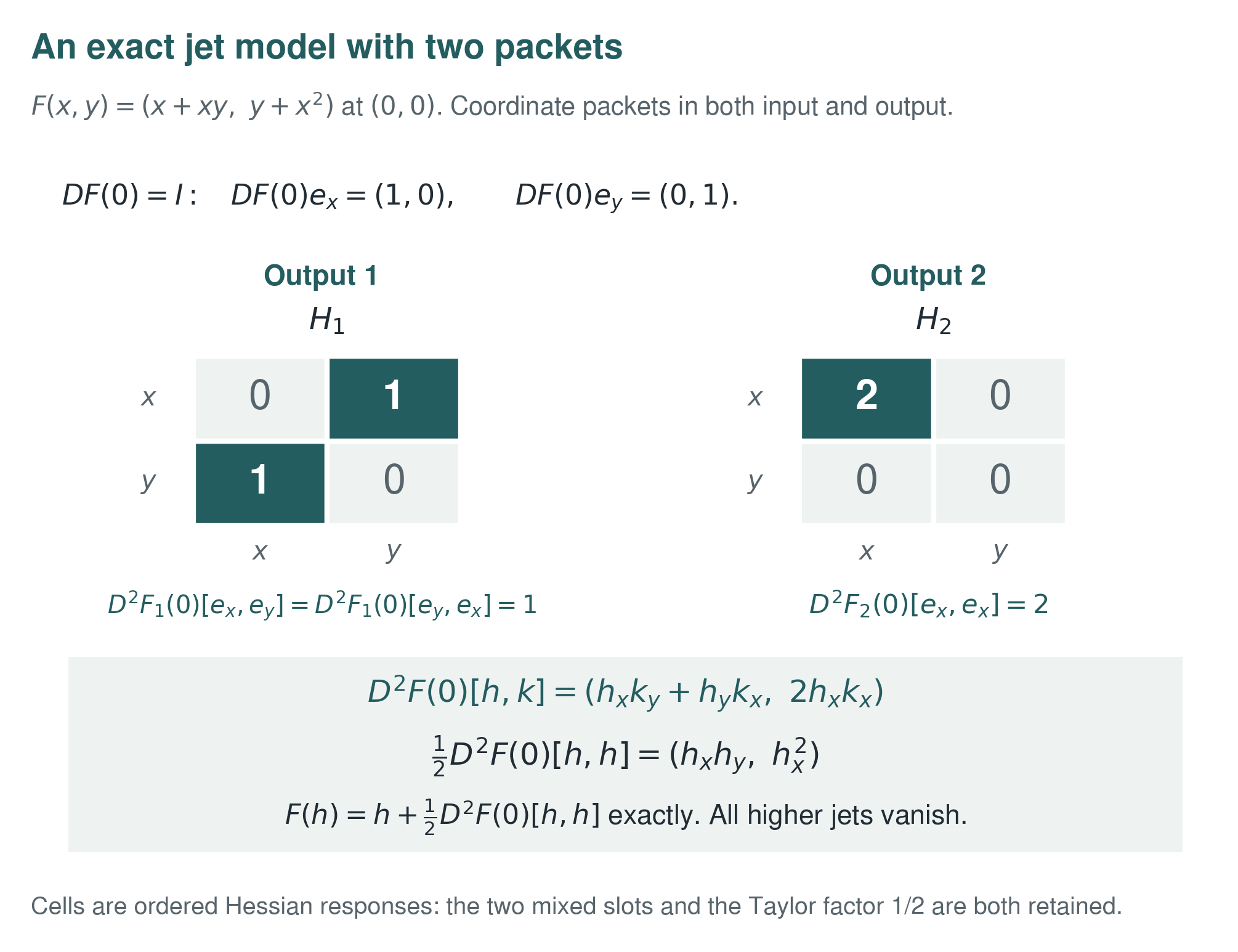
At the origin, the two output Hessians of F(x,y)=(x+xy,y+x squared) are [zero, one; one, zero] and [two, zero; zero, zero]. — Second packet jets for \(F(x,y)=(x+xy,y+x^2)\) at the origin. Coordinate axis projectors give \(DF(0)=I\). The first output has mixed second derivatives equal to one, while the second has a repeated first input derivative equal to two. Each grid records the ordered pair of input packets. The mixed entries retain an interaction that diagonal restrictions would lose.

Proposition 17.3: Jet norm bound

Give every packet range its inherited subspace norm. The restricted jet satisfies the sharper estimate

\[ \left\|J^r_{\gamma\mid\alpha_1,\ldots,\alpha_r}F(x)\right\| \le \|Q_\gamma\|\,\|D^rF(x)\|. \]

Its ambient extension inserts \(P_{\alpha_j}\) in the \(j\)th slot and has norm at most \(\|Q_\gamma\|\,\|D^rF(x)\|\prod_j\|P_{\alpha_j}\|\). Consequently the operator norm of the restricted packet jet also satisfies

\[ \left\|J^{r}_{\gamma\mid\alpha_1,\ldots,\alpha_r}F(x)\right\| \le \|Q_\gamma\|\,\|D^rF(x)\| \prod_{j=1}^r\|P_{\alpha_j}\|. \]

When all packets are orthogonal projections on Hilbert spaces, every nonzero projector has norm one and the bound reduces to the norm of the full derivative.

Read proof · Read statement and proof side by side · Permalink · Source line 258 · Claim record · Lean coverage · Code · Worked examples

Proof of Proposition 17.3

For \(h_j\in X_{\alpha_j}\), the inherited norm gives

\[ \|Q_\gamma D^rF(x)[h_1,\ldots,h_r]\| \le \|Q_\gamma\|\,\|D^rF(x)\|\prod_j\|h_j\|. \]

Taking the multilinear operator norm proves the sharper restricted estimate. For ambient inputs, replace \(h_j\) by \(P_{\alpha_j}h_j\) and apply the operator norm bound to each projector. Every nonzero idempotent has norm at least one, since it fixes a nonzero vector in its range. The displayed product bound therefore also follows for the restricted jet. If a zero packet is retained as a redundant index, multilinearity makes any jet with that input or output packet zero, so both estimates remain valid.

Back to statement · Read statement and proof side by side · Permalink · Source line 276 · Claim record · Lean coverage · Code · Worked examples

Corollary 17.4: Packet Taylor formula

Assume \(F\) is \(m+1\) times continuously Fréchet differentiable on an open set containing the segment \(x+th\) for \(0\le t\le1\). Then

\[ \begin{aligned} Q_\gamma F(x+h) ={}&Q_\gamma F(x) + \sum_{r=1}^{m}\frac1{r!} \sum_{\alpha_1,\ldots,\alpha_r} J^{r}_{\gamma\mid\alpha_1,\ldots,\alpha_r}F(x) [P_{\alpha_1}h,\ldots,P_{\alpha_r}h]\\ &+Q_\gamma R_{m+1}(x,h), \end{aligned} \]

where the Bochner integral remainder is

\[ R_{m+1}(x,h) = \frac1{m!} \int_0^1(1-t)^m D^{m+1}F(x+th)[h,\ldots,h]\,dt. \]

Read proof · Read statement and proof side by side · Permalink · Source line 285 · Claim record · Lean coverage · Code · Worked examples

Proof of Corollary 17.4

Set \(g(t)=F(x+th)\) on the open preimage of the domain under \(t\mapsto x+th\). It contains \([0,1]\), and repeated differentiation gives \(g^{(r)}(t)=D^rF(x+th)[h,\ldots,h]\). The derivatives are continuous on the compact interval, so their Bochner integrals exist in the Banach codomain. Put

\[ T_j=\frac1{j!}\int_0^1(1-t)^j g^{(j+1)}(t)\,dt \qquad(0\le j\le m). \]

The fundamental theorem of calculus gives \(T_0=g(1)-g(0)\). For \(j\ge1\), integration by parts gives \(T_j=T_{j-1}-g^{(j)}(0)/j!\). Iterating this relation proves the Taylor identity with remainder \(T_m=R_{m+1}(x,h)\) and its exact factorial normalization.

Apply \(Q_\gamma\) to the identity and use Theorem 17.2. Pairwise annihilation and idempotence retain exactly the output packet \(\gamma\). Boundedness of \(Q_\gamma\) allows it to pass through the Bochner integral. In particular, if \(\|D^{m+1}F(x+th)\|\le M\) along the segment, then

\[ \|Q_\gamma R_{m+1}(x,h)\| \le \frac{\|Q_\gamma\|M\|h\|^{m+1}}{(m+1)!}. \]

For \(m=0\) the Taylor sum is empty. For \(h=0\), multilinearity makes every positive-order term and the remainder zero.

Back to statement · Read statement and proof side by side · Permalink · Source line 309 · Claim record · Lean coverage · Code · Worked examples

The relation to derivatives of the complete coordinate representation is also literal. For an open domain \(U\subseteq X\), put \(\widehat F={\mathcal A}_{{\mathcal Q}}\circ F\circ{\mathcal S}_{{\mathcal P}}\) on the open coordinate set \({\mathcal A}_{{\mathcal P}}(U)\). Boundedness and linearity of analysis and synthesis imply, for \(1\le r\le m\),

\[ D^r\widehat F(u)[v_1,\ldots,v_r] ={\mathcal A}_{{\mathcal Q}}\bigl(D^rF({\mathcal S}_{{\mathcal P}}u) [{\mathcal S}_{{\mathcal P}}v_1,\ldots,{\mathcal S}_{{\mathcal P}}v_r]\bigr). \]

Indeed, the first derivative follows from the chain rule. Repeating it adds no higher derivatives of the fixed linear coordinate maps. If each \(v_j\) is supported in one coordinate slot \(\alpha_j\), synthesis includes that slot into \(X\). Its \(\gamma\) output component is exactly the range jet defined above, including when a chosen direction is zero.

At a fixed base point, the nonzero packet jets form a directed hypergraph. An order \(r\) interaction has \(r\) input packet labels and one output packet label. The support therefore records interactions relative to the chosen packet system.

For a block \(B=\{i_1<\cdots<i_s\}\) and an intermediate packet \(\gamma\), write

\[ G_{\gamma,B}(x\mid h) = J^s_{\gamma\mid\alpha_{i_1},\ldots,\alpha_{i_s}}G(x) [h_{i_1},\ldots,h_{i_s}]. \]

Permalink · Source line 328

Arity of packet jets

A packet jet has one output slot and as many input slots as its derivative order. In the composition formula, each partition block collects inputs for one derivative of the inner map. The number of blocks determines the arity of the derivative of the outer map. Intermediate packet labels record the outputs passed between them.

Permalink · Source line 347

Theorem 17.5: Packet Faà di Bruno formula

Let \(n\ge1\), let \(X,Y,Z\) be Banach spaces over the same real or complex field, and let \(G:X\to Y\) and \(F:Y\to Z\) be \(n\) times continuously Fréchet differentiable. Let \({\mathcal P}\), \({\mathcal Q}\), and \({\mathcal R}\) be packet systems on \(X\), \(Y\), and \(Z\). Fix input packets \(\alpha_1,\ldots,\alpha_n\), an output packet \(\delta\), and directions \(h_i\in X_{\alpha_i}\). Then

\[ \begin{aligned} &J^{n}_{\delta\mid\alpha_1,\ldots,\alpha_n}(F\circ G)(x) [h_1,\ldots,h_n]\\ &= \sum_{\pi=\{B_1,\ldots,B_k\}} \sum_{\gamma_1,\ldots,\gamma_k} J^{k}_{\delta\mid\gamma_1,\ldots,\gamma_k}F(Gx) \big[ G_{\gamma_1,B_1}(x\mid h),\ldots, G_{\gamma_k,B_k}(x\mid h) \big]. \end{aligned} \]

The first sum runs over all set partitions of \(\{1,\ldots,n\}\).

Read proof · Read statement and proof side by side · Permalink · Source line 351 · Claim record · Lean coverage · Code · Worked examples

Proof of Theorem 17.5

First derive the unprojected partition formula. At order one it is the ordinary chain rule. Suppose it holds at order \(n\) and the maps are \(C^{n+1}\). Differentiating a summand in direction \(h_{n+1}\) has two kinds of contribution. A derivative of the outer map creates the new singleton block \(\{n+1\}\). A derivative of an inner block jet adjoins \(n+1\) to that block. Every partition of \(\{1,\ldots,n+1\}\) arises exactly once: if \(\{n+1\}\) is a block, remove that block. Otherwise remove \(n+1\) from the unique block that contains it. The chain and product rules for bounded multilinear evaluation justify the differentiation. This proves the unprojected formula by induction.

Insert \(I_Y=\sum_\gamma Q_\gamma\) in each argument of the outer derivative and expand the finite sums by multilinearity. Apply \(R_\delta\) to the output. The directions already lie in the declared input ranges, and each intermediate projection lands in its literal output range. The resulting summands are exactly the displayed packet jets. List directions within a block in increasing index order and blocks in increasing least-element order. Symmetry of the higher derivative makes the final value independent of the block ordering.

Back to statement · Read statement and proof side by side · Permalink · Source line 370 · Claim record · Lean coverage · Code · Worked examples

Proposition 17.6: Number of labeled composition terms

For \(n\ge1\), if \(Y\) has \(M\) packets, then the number of packet labeled terms at order \(n\) before zero jets are removed is

\[ N_{n,M} = \sum_{k=1}^{n}S(n,k)M^k, \]

where \(S(n,k)\) is a Stirling number of the second kind. Thus \(N_{n,M}\) is the \(n\)th Touchard polynomial evaluated at \(M\).

Read proof · Read statement and proof side by side · Permalink · Source line 376 · Claim record · Lean coverage · Code · Worked examples

Proof of Proposition 17.6

A set partition with \(k\) blocks receives one independent intermediate packet label on each block. It therefore gives \(M^k\) labeled terms. There are \(S(n,k)\) such partitions.

Back to statement · Read statement and proof side by side · Permalink · Source line 386 · Claim record · Lean coverage · Code · Worked examples

Corollary 17.7: Structural pruning

For a map \(H\) with fixed input and output packet systems, let \({\operatorname{supp}}_r H(x)\) be the set of external profiles \((\delta;\alpha_1,\ldots,\alpha_r)\) for which the restricted jet \(J^r_{\delta\mid\alpha_1,\ldots,\alpha_r}H(x)\) is nonzero. A profile belongs to the admissible composition set if it admits a partition \(\pi=\{B_1,\ldots,B_k\}\) and intermediate labels \(\gamma_1,\ldots,\gamma_k\) such that the outer jet of \(F\) and every inner block jet of \(G\) in Theorem 17.5 are nonzero. Then \({\operatorname{supp}}_n(F\circ G)(x)\) is contained in this admissible set. In particular, a summand vanishes whenever one of its constituent packet jets vanishes.

Read proof · Read statement and proof side by side · Permalink · Source line 390 · Claim record · Lean coverage · Code · Worked examples

Proof of Corollary 17.7

If a profile has no admissible decorated partition, every summand in Theorem 17.5 has a zero constituent and therefore vanishes. The composed jet is then the zero multilinear map. This proves the support inclusion by contraposition. The inclusion can be strict. Nonzero constituent maps may compose to zero, and nonzero summands may cancel. Thus the admissible set is a structural upper bound rather than a claim of equality.

Back to statement · Read statement and proof side by side · Permalink · Source line 394 · Claim record · Lean coverage · Code · Worked examples

Example 17.8: The second order composition law

At order two, the partition formula has two shapes. For packet directions \(h_1\) and \(h_2\),

\[ \begin{aligned} R_\delta D^2(F\circ G)(x)[h_1,h_2] ={}& \sum_{\gamma_1,\gamma_2} J^2_{\delta\mid\gamma_1,\gamma_2}F(Gx) [J^1_{\gamma_1\mid\alpha_1}G(x)h_1,J^1_{\gamma_2\mid\alpha_2}G(x)h_2]\\ &+ \sum_\gamma J^1_{\delta\mid\gamma}F(Gx) [J^2_{\gamma\mid\alpha_1,\alpha_2}G(x)[h_1,h_2]]. \end{aligned} \]

The first line records two first order changes entering a quadratic interaction of \(F\). The second records a genuine second order interaction created inside \(G\) before \(F\) is applied.

Permalink · Source line 399

Remark 17.9

Jet sparsity is not invariant under an arbitrary change of coordinates. A useful packet system normally comes from symmetry, scale, support, grading, valuation, or another structure that is already present in the problem. Every sparsity claim should therefore name the packet system with respect to which it is made.

Permalink · Source line 417

18 Rooted tree expansions

On this page · Permalink · Source line 421

Repeated nonlinear substitution is indexed by rooted trees. We begin with a polynomial fixed point equation on a Banach space.

Let \(X\) be a Banach space. Fix \(s\in X\) and continuous multilinear maps

\[ B_r:X^r\longrightarrow X, \qquad 2\le r\le d. \]

Set

\[ a=\|s\|, \qquad b_r=\|B_r\|, \qquad \phi(t)=a+\sum_{r=2}^{d}b_rt^r. \]

An ordered rooted tree has leaves labeled by \(s\) and every internal vertex of arity \(r\) labeled by \(B_r\). Its value is obtained by evaluating from the leaves toward the root.

Permalink · Source line 423

Theorem 18.1: Polynomial tree expansion

Suppose there is \(R>0\) such that

\[ \phi(R)\le R \]

and

\[ q= \sum_{r=2}^{d}r b_rR^{r-1}<1. \]

Then the map

\[ \Phi(x)=s+\sum_{r=2}^{d}B_r(x,\ldots,x) \]

has a unique fixed point in the closed ball \(\overline B_R(0)\). The sum of the values of all finite ordered rooted trees converges absolutely to that fixed point.

Read proof · Read statement and proof side by side · Permalink · Source line 441 · Claim record · Lean coverage · Code · Worked examples

Proof of Theorem 18.1

For \(x,y\in\overline B_R(0)\), multilinearity and telescoping in the \(r\) input positions give

\[ \|B_r(x,\ldots,x)-B_r(y,\ldots,y)\| \le r b_rR^{r-1}\|x-y\|. \]

Hence \(\Phi\) is \(q\) Lipschitz on the ball. The inequality \(\phi(R)\le R\) shows that \(\Phi\) preserves the ball. The contraction mapping theorem gives a unique fixed point \(u\) in that ball.

Let \(\mathfrak T_m\) be the finite set of ordered rooted trees of height less than \(m\). A leaf has value \(s\). If the root of \(\tau\) has arity \(r\) and ordered subtrees \(\tau_1,\ldots,\tau_r\), define

\[ B_\tau(s)=B_r(B_{\tau_1}(s),\ldots,B_{\tau_r}(s)). \]

Induction on \(m\) shows that the Picard iterate \(u_0=0\) and \(u_{m+1}=\Phi(u_m)\) satisfies

\[ u_m=\sum_{\tau\in\mathfrak T_m}B_\tau(s). \]

Define a nonnegative scalar weight by assigning weight \(a\) to a leaf and applying the scalar map \((t_1,\ldots,t_r)\mapsto b_rt_1\cdots t_r\) at a vertex of arity \(r\). A second induction gives

\[ \sum_{\tau\in\mathfrak T_m}\|B_\tau(s)\| \le \sum_{\tau\in\mathfrak T_m}w(\tau) =t_m, \]

where \(t_0=0\) and \(t_{m+1}=\phi(t_m)\). The sequence \((t_m)\) is increasing because \(\phi\) has nonnegative coefficients. It is bounded by \(R\) because \(t_0\le R\) and \(\phi(R)\le R\). The sum of the norms of all tree values is therefore finite. The tree series converges absolutely. Its partial sums are the Picard iterates, so its sum is \(u\).

Back to statement · Read statement and proof side by side · Permalink · Source line 458 · Claim record · Lean coverage · Code · Worked examples

Corollary 18.2: Quadratic Catalan expansion

Let \(B:X\times X\to X\) be bounded and consider

\[ u=s+B(u,u). \]

Put \(a=\|s\|\) and \(b=\|B\|\). If \(4ab<1\), then

\[ u= \sum_{n\ge1} \sum_{\substack{\tau\text{ full ordered binary tree}\\\text{with }n\text{ leaves}}} B_\tau(s) \]

converges absolutely. It also satisfies

\[ \|u\| \le \frac{1-\sqrt{1-4ab}}{2b} \]

when \(b>0\).

Read proof · Read statement and proof side by side · Permalink · Source line 485 · Claim record · Lean coverage · Code · Worked examples

Proof of Corollary 18.2

If \(b=0\), the equation is \(u=s\) and the tree series contains only its one leaf. If \(a=0\), every tree value is zero. Choose any \(R\) with \(0<R<1/(2b)\) and apply Theorem 18.1 to obtain uniqueness of the zero fixed point in that ball.

Assume now that \(a>0\) and \(b>0\). Take

\[ R= \frac{1-\sqrt{1-4ab}}{2b}. \]

Then \(a+bR^2=R\) and \(2bR<1\). Apply Theorem 18.1. The number of full ordered binary trees with \(n\) leaves is the Catalan number \(C_{n-1}\), which gives the displayed majorant.

Back to statement · Read statement and proof side by side · Permalink · Source line 506 · Claim record · Lean coverage · Code · Worked examples

Theorem 18.3: Packet labeled tree reconstruction

Let \(X\) carry a packet system \({\mathcal P}\). At each internal vertex of a tree, insert the output identity and one input identity for every child. Summing over all internal packet labels reconstructs the original tree value exactly.

Read proof · Visual guide: Mixed terms are not optional · Read statement and proof side by side · Permalink · Source line 517 · Claim record · Lean coverage · Code · Worked examples

Proof of Theorem 18.3

At a vertex labeled by an \(r\) multilinear map \(B_r\), insert

\[ I_X=\sum_\beta P_\beta \]

on the output and in every input slot. Multilinearity gives an exact finite sum of packet blocks at that vertex. Apply this identity successively from the leaves toward the root. Since the tree and the packet set are finite, all sums are finite and their total reconstructs the original tree value.

Back to statement · Read statement and proof side by side · Permalink · Source line 521 · Claim record · Lean coverage · Code · Worked examples

For an infinite tree expansion, the finite sum of packet decorations for each underlying tree is kept together. The unlabelled tree majorant does not imply absolute convergence when all decorations are summed separately for arbitrary oblique projectors. Finite tree reconstruction and the grouped interpretation remain exact.

Permalink · Source line 529

Arity in a tree

At each internal vertex, the number of children is the number of input slots of its multilinear map. Their order is retained because symmetry is not assumed. Packet labels resolve each finite tree into a finite sum. In an infinite expansion these sums stay grouped by tree, as required by the convergence statement above.

Permalink · Source line 531

Corollary 18.4: Tree pruning

A packet labeled tree vanishes if one internal vertex carries a zero packet block of the corresponding multilinear map. Removing all such zero terms leaves every finite tree sum unchanged and therefore leaves the grouped infinite series unchanged.

Read proof · Read statement and proof side by side · Permalink · Source line 535 · Claim record · Lean coverage · Code · Worked examples

Proof of Corollary 18.4

A zero vertex map makes the value of the full tree zero.

Back to statement · Read statement and proof side by side · Permalink · Source line 539 · Claim record · Lean coverage · Code · Worked examples

The tree theorem separates combinatorial growth from analytic convergence. The number of trees may grow rapidly, while multilinear bounds control their values. The scalar map \(\phi\) controls the total weight of the expansion. Packet pruning changes the combinatorics but not the proof. It removes trees whose values are already zero before any norm estimate is used.

Permalink · Source line 544

Example 18.5: Catalan parity packets

Over a field of characteristic zero, the formal equation

\[ u=z+u^2 \]

has the branch

\[ u(z)=\frac{1-\sqrt{1-4z}}2. \]

Write \(u=u_0+u_1\), where \(u_0\) contains the even powers of \(z\) and \(u_1\) contains the odd powers. Exact packet projection gives

\[ u_0=u_0^2+u_1^2, \qquad u_1=z+2u_0u_1. \]

The two equations remain coupled. Their sum is the original fixed point equation.

Permalink · Source line 546

19 Graded nonlinear operations

On this page · Permalink · Source line 564

Let \(G\) be a finite abelian group and let

\[ A=\bigoplus_{g\in G}A_g \]

be a \(G\) graded module.

Permalink · Source line 566

Definition 19.1: Grade respecting operation

An \(r\) multilinear map \(\mu:A^r\to A\) respects the grading when

\[ \mu(A_{g_1},\ldots,A_{g_r}) \subseteq A_{g_1+\cdots+g_r}. \]

Permalink · Source line 572 · Claim record · Lean coverage · Code · Worked examples

Theorem 19.2: Graded packet convolution

If \(a_j=\sum_{g\in G}a_{j,g}\) and \(\mu\) respects the grading, then

\[ P_k\mu(a_1,\ldots,a_r) = \sum_{g_1+\cdots+g_r=k} \mu(a_{1,g_1},\ldots,a_{r,g_r}). \]

Read proof · Read statement and proof side by side · Permalink · Source line 581 · Claim record · Lean coverage · Code · Worked examples

Proof of Theorem 19.2

Expand every input into its homogeneous components. Each term lands in the component whose label is the sum of its input labels. Projection onto \(A_k\) retains exactly the displayed terms.

Back to statement · Read statement and proof side by side · Permalink · Source line 591 · Claim record · Lean coverage · Code · Worked examples

Corollary 19.3: Cyclic product formula

For a cyclically graded algebra

\[ A=\bigoplus_{j\in\mathbb Z/N\mathbb Z}A_j, \qquad A_iA_j\subseteq A_{i+j}, \]

one has

\[ P_k(ab)= \sum_{i+j=k}a_ib_j. \]

Read proof · Read statement and proof side by side · Permalink · Source line 595 · Claim record · Lean coverage · Code · Worked examples

Proof of Corollary 19.3

Apply Theorem 19.2 to multiplication.

Back to statement · Read statement and proof side by side · Permalink · Source line 609 · Claim record · Lean coverage · Code · Worked examples

Theorem 19.4: Packet Maurer Cartan equations

Let

\[ {\mathcal L}=\bigoplus_{g\in G}{\mathcal L}_g \]

be a differential graded Lie algebra over a ring in which two is invertible. Assume

\[ d{\mathcal L}_g\subseteq{\mathcal L}_g, \qquad [{\mathcal L}_g,{\mathcal L}_h]\subseteq{\mathcal L}_{g+h}. \]

For a degree one element \(\eta=\sum_g\eta_g\), the Maurer Cartan equation

\[ d\eta+\frac12[\eta,\eta]=0 \]

is equivalent to

\[ d\eta_k + \frac12 \sum_{g+h=k}[\eta_g,\eta_h] =0 \]

for every \(k\in G\).

Read proof · Read statement and proof side by side · Permalink · Source line 613 · Claim record · Lean coverage · Code · Worked examples

Proof of Theorem 19.4

The differential preserves the group label and the bracket adds labels. Apply the projector onto \({\mathcal L}_k\) and use exact reconstruction.

Back to statement · Read statement and proof side by side · Permalink · Source line 639 · Claim record · Lean coverage · Code · Worked examples

The same argument applies to higher brackets.

Permalink · Source line 643

Proposition 19.5: Packet equations for \(L_\infty\) operations

Let \({\mathcal L}\) be complete and carry operations \(\ell_r\) that respect a finite abelian group grading. Assume the packet projectors are continuous for the topology in which the series below converges. Assume the Maurer Cartan series

\[ \sum_{r\ge1}\frac1{r!}\ell_r(\eta,\ldots,\eta) \]

converges and the required factorials are invertible. Then its packet of label \(k\) is

\[ \sum_{r\ge1}\frac1{r!} \sum_{g_1+\cdots+g_r=k} \ell_r(\eta_{g_1},\ldots,\eta_{g_r}). \]

The full Maurer Cartan equation holds if and only if every packet equation vanishes.

Read proof · Read statement and proof side by side · Permalink · Source line 645 · Claim record · Lean coverage · Code · Worked examples

Proof of Proposition 19.5

Apply Theorem 19.2 to each operation \(\ell_r\). Continuity of the packet projectors permits the convergent sums to be projected term by term.

Back to statement · Read statement and proof side by side · Permalink · Source line 659 · Claim record · Lean coverage · Code · Worked examples

Definition 19.6: Divided square

A divided square on degree one elements is a map \(q\) satisfying

\[ q(x+y)=q(x)+q(y)+[x,y], \qquad q(ax)=a^2q(x), \]

whenever the expressions are defined.

Permalink · Source line 663 · Claim record · Lean coverage · Code · Worked examples

Proposition 19.7: Divided square packet equations

Assume \(q({\mathcal L}_g)\subseteq{\mathcal L}_{2g}\). Choose an ordering of the finite label set. The equation

\[ d\eta+q(\eta)=0 \]

is equivalent to

\[ d\eta_k + \sum_{2g=k}q(\eta_g) + \sum_{\substack{g<h\\g+h=k}}[\eta_g,\eta_h] =0 \]

for every \(k\).

Read proof · Read statement and proof side by side · Permalink · Source line 673 · Claim record · Lean coverage · Code · Worked examples

Proof of Proposition 19.7

Repeated use of the polarization identity for \(q\) gives

\[ q\left(\sum_g\eta_g\right) = \sum_gq(\eta_g) + \sum_{g<h}[\eta_g,\eta_h]. \]

Project onto the component of label \(k\).

Back to statement · Read statement and proof side by side · Permalink · Source line 690 · Claim record · Lean coverage · Code · Worked examples

Example 19.8: Matrix difference grading

Let \(A=M_N({\Bbbk})\) and assign the matrix unit \(E_{rs}\) the label \(r-s\) modulo \(N\). Since

\[ E_{rs}E_{uv}=\delta_{su}E_{rv}, \]

the output label is

\[ (r-s)+(u-v)=r-v \]

whenever the product is nonzero. Matrix multiplication therefore obeys the cyclic convolution law exactly. The same grading resolves commutators and polynomial matrix equations.

Permalink · Source line 703

Remark 19.9

These results begin with a graded differential or higher algebra. They do not assert that every deformation problem has such a controlling object. Differential graded and infinity algebra methods are developed in [LodayVallette2012].

Permalink · Source line 715

20 Nonlinear refinement defects

On this page · Permalink · Source line 719

Let

\[ F_f:X_f\longrightarrow Y_f, \qquad F_c:X_c\longrightarrow Y_c \]

be fine and coarse maps. Let

\[ C_X:X_f\longrightarrow X_c, \qquad C_Y:Y_f\longrightarrow Y_c \]

be linear coarsening maps. Whenever a norm, a Lipschitz constant, or a Fréchet derivative is used, the spaces are Banach spaces and the coarsening maps are bounded.

Permalink · Source line 721

Definition 20.1: Nonlinear refinement defect

The pointwise defect of \(F\) is

\[ \Delta_F(x) = C_YF_f(x)-F_c(C_Xx). \]

The two models are exactly compatible when \(\Delta_F\) vanishes everywhere.

Permalink · Source line 735 · Claim record · Lean coverage · Code · Worked examples

The defect is a vector in \(Y_c\). It determines an obstruction class after a correction map into \(Y_c\) has been chosen and the defect has been passed to the corresponding cokernel. Norm estimates measure the size of the defect. The quotient determines whether an allowed linear correction can remove it.

Permalink · Source line 746

Theorem 20.2: Exact defect under composition

Let \(G_f:Y_f\to Z_f\) and \(G_c:Y_c\to Z_c\), with coarsening \(C_Z:Z_f\to Z_c\). Then

\[ \Delta_{G\circ F}(x) = \Delta_G(F_f(x)) + G_c\big(F_c(C_Xx)+\Delta_F(x)\big) - G_c\big(F_c(C_Xx)\big). \]

If \(G_c\) is \(L\) Lipschitz on the relevant set, then

\[ \|\Delta_{G\circ F}(x)\| \le \|\Delta_G(F_f(x))\| + L\|\Delta_F(x)\|. \]

Read proof · Visual guide: Where a nonlinear defect can enter · Read statement and proof side by side · Permalink · Source line 748 · Claim record · Lean coverage · Code · Worked examples

Proof of Theorem 20.2

Add and subtract \(G_c(C_YF_f(x))\). Use

\[ C_YF_f(x)=F_c(C_Xx)+\Delta_F(x). \]

The norm estimate follows from the Lipschitz bound.

Back to statement · Read statement and proof side by side · Permalink · Source line 769 · Claim record · Lean coverage · Code · Worked examples

Corollary 20.3: Linear product rule

If all maps in Theorem 20.2 are linear, then

\[ \Delta_{GF} = \Delta_G F_f+G_c\Delta_F. \]

Read proof · Read statement and proof side by side · Permalink · Source line 777 · Claim record · Lean coverage · Code · Worked examples

Proof of Corollary 20.3

Linearity turns the last difference in Theorem 20.2 into \(G_c\Delta_F(x)\).

Back to statement · Read statement and proof side by side · Permalink · Source line 786 · Claim record · Lean coverage · Code · Worked examples

Theorem 20.4: Iterated orbit defect

Let \(F_f:X_f\to X_f\) and \(F_c:X_c\to X_c\), with coarsening \(C:X_f\to X_c\). Suppose \(F_c\) is \(q\) Lipschitz. For a fine orbit starting at \(x\), assume

\[ \|\Delta_F(F_f^j x)\|\le\varepsilon_j. \]

Then

\[ \left\|CF_f^n(x)-F_c^n(Cx)\right\| \le \sum_{j=0}^{n-1}q^{n-1-j}\varepsilon_j. \]

If \(0\le q<1\) and every \(\varepsilon_j\le\varepsilon\), then

\[ \left\|CF_f^n(x)-F_c^n(Cx)\right\| \le \varepsilon\frac{1-q^n}{1-q}. \]

Read proof · Read statement and proof side by side · Permalink · Source line 790 · Claim record · Lean coverage · Code · Worked examples

Proof of Theorem 20.4

Let

\[ e_n=\left\|CF_f^n(x)-F_c^n(Cx)\right\|. \]

The definition of the defect and the Lipschitz property give

\[ e_{n+1}\le\varepsilon_n+qe_n. \]

Iterating this recurrence proves the first estimate. The second is the geometric sum.

Back to statement · Read statement and proof side by side · Permalink · Source line 809 · Claim record · Lean coverage · Code · Worked examples

Theorem 20.5: Fixed point stability

Assume \(F_c\) is a contraction with constant \(q<1\). Let \(x_f\) and \(x_c\) be fixed points of \(F_f\) and \(F_c\). If

\[ \|\Delta_F(x_f)\|\le\varepsilon, \]

then

\[ \|Cx_f-x_c\| \le \frac{\varepsilon}{1-q}. \]

When the defect at \(x_f\) is zero, the fixed points are compatible.

Read proof · Read statement and proof side by side · Permalink · Source line 821 · Claim record · Lean coverage · Code · Worked examples

Proof of Theorem 20.5

Using the fixed point equations,

\[ \begin{aligned} \|Cx_f-x_c\| &\le \|CF_f(x_f)-F_c(Cx_f)\| + \|F_c(Cx_f)-F_c(x_c)\|\\ &\le \varepsilon+q\|Cx_f-x_c\|. \end{aligned} \]

Rearrange.

Back to statement · Read statement and proof side by side · Permalink · Source line 835 · Claim record · Lean coverage · Code · Worked examples

Corollary 20.6: Several refinement levels

Let \(C_\ell:X_{\ell+1}\to X_\ell\) for \(0\le\ell<m\). Suppose \(x_\ell\) is a fixed point at level \(\ell\), the coarse map at level \(\ell\) has contraction constant \(q_\ell<1\), and the adjacent defect at \(x_{\ell+1}\) is at most \(\varepsilon_\ell\). Write

\[ C_{a,b}=C_aC_{a+1}\cdots C_{b-1} \quad\text{for }a<b, \qquad C_{a,a}=I. \]

Then

\[ \|C_{0,m}x_m-x_0\| \le \sum_{\ell=0}^{m-1} \|C_{0,\ell}\| \frac{\varepsilon_\ell}{1-q_\ell}. \]

Read proof · Read statement and proof side by side · Permalink · Source line 851 · Claim record · Lean coverage · Code · Worked examples

Proof of Corollary 20.6

Insert the intermediate vectors \(C_{0,\ell}x_\ell\) and telescope. Apply Theorem 20.5 to every adjacent pair.

Back to statement · Read statement and proof side by side · Permalink · Source line 869 · Claim record · Lean coverage · Code · Worked examples

Proposition 20.7: Derivative defects

Assume \(F_f\) and \(F_c\) are \(r\) times Fréchet differentiable and the coarsening maps are bounded and linear. Then

\[ D\Delta_F(x) = C_YDF_f(x)-DF_c(C_Xx)C_X. \]

For \(r\ge2\),

\[ D^r\Delta_F(x)[h_1,\ldots,h_r] = C_YD^rF_f(x)[h_1,\ldots,h_r] - D^rF_c(C_Xx)[C_Xh_1,\ldots,C_Xh_r]. \]

Read proof · Read statement and proof side by side · Permalink · Source line 873 · Claim record · Lean coverage · Code · Worked examples

Proof of Proposition 20.7

Differentiate the defining identity for \(\Delta_F\). The coarsening maps are linear, so their higher derivatives vanish.

Back to statement · Read statement and proof side by side · Permalink · Source line 890 · Claim record · Lean coverage · Code · Worked examples

Example 20.8: Sharp affine bound

Let \(F_c(y)=qy+b\) with \(0<q<1\). Choose a fine fixed point whose coarsening has constant defect \(\varepsilon\) in the direction of the scalar state. The fixed point mismatch is exactly \(\varepsilon/(1-q)\). Thus the constant in Theorem 20.5 cannot be improved without more information.

Permalink · Source line 894

21 Canonical obstruction objects

On this page · Permalink · Source line 898

We begin by isolating the part of a defect that cannot be removed by an allowed linear correction.

Permalink · Source line 900

Definition 21.1: Linear correction datum

A linear correction datum consists of a homomorphism

\[ D:U\longrightarrow V \]

and a defect \(r\in V\). A correction is an element \(u\in U\) satisfying

\[ Du=-r. \]

The obstruction class is

\[ {\operatorname{Ob}}_D(r)=[r]\in{\operatorname{coker}} D=V/{\operatorname{im}} D. \]

Permalink · Source line 902 · Claim record · Lean coverage · Code · Worked examples

Theorem 21.2: Cokernel obstruction criterion

A linear correction exists if and only if

\[ {\operatorname{Ob}}_D(r)=0. \]

The quotient map

\[ q_D:V\longrightarrow{\operatorname{coker}} D \]

has the following universal property. If \(\varphi:V\to W\) is linear and \(\varphi D=0\), then there is a unique linear map

\[ \overline\varphi:{\operatorname{coker}} D\longrightarrow W \]

with \(\varphi=\overline\varphi q_D\).

Read proof · Read statement and proof side by side · Permalink · Source line 917 · Claim record · Lean coverage · Code · Worked examples

Proof of Theorem 21.2

The class of \(r\) is zero exactly when \(r\in{\operatorname{im}} D\), which is equivalent to solvability of \(Du=-r\). If \(\varphi D=0\), then \(\varphi\) vanishes on \({\operatorname{im}} D\). It therefore descends uniquely to the quotient.

Back to statement · Read statement and proof side by side · Permalink · Source line 933 · Claim record · Lean coverage · Code · Worked examples

The universal property explains why the cokernel is the canonical obstruction object relative to \(D\). Any linear obstruction test that vanishes on correctable defects factors through it.

Permalink · Source line 937

Canonical obstruction data

The residual, the correction map, and the obstruction class are distinct data. The residual is a vector. The correction map specifies which changes are allowed, and its cokernel records the remaining class. Canonicality is relative to that declared correction map. A scalar or orthogonal representative of the class may require further choices or hypotheses.

Permalink · Source line 939

The defect (two, three) splits into a horizontal correctable part (two, zero) and a remaining vertical representative (zero, three). — A specified correction range in \(\mathbb R^2\). For \(L(a,b)=(a,0)\), the image is the horizontal axis. The defect \((2,3)\) splits into \((2,0)\) in that image and the remaining representative \((0,3)\). Subtracting the image component leaves the same cokernel class. The functional \((x,y)\mapsto y\) vanishes on the correction range and detects the value three. The correction equation \(Lu=-(2,3)\) therefore has no solution.

Theorem 21.3: Naturality of obstruction classes

Suppose

\[ \begin{array}{ccc} U & \xrightarrow{D} & V\\ \mathllap{a}\downarrow & & \downarrow\mathrlap{b}\\ U' & \xrightarrow{D'} & V' \end{array} \]

is a commuting square. Then there is a unique induced map

\[ \overline b:{\operatorname{coker}} D\longrightarrow{\operatorname{coker}} D' \]

satisfying

\[ \overline b\,{\operatorname{Ob}}_D(r)={\operatorname{Ob}}_{D'}(br). \]

Read proof · Read statement and proof side by side · Permalink · Source line 951 · Claim record · Lean coverage · Code · Worked examples

Proof of Theorem 21.3

The relation \(bD=D'a\) shows that the quotient map \(q_{D'}b\) vanishes on \({\operatorname{im}} D\). Apply the universal property in Theorem 21.2.

Back to statement · Read statement and proof side by side · Permalink · Source line 970 · Claim record · Lean coverage · Code · Worked examples

Theorem 21.4: Packet decomposition of an obstruction

Suppose

\[ U=\bigoplus_{\alpha\in I}U_\alpha, \qquad V=\bigoplus_{\alpha\in I}V_\alpha, \]

and \(D(U_\alpha)\subseteq V_\alpha\) for every \(\alpha\). Let

\[ D_\alpha:U_\alpha\longrightarrow V_\alpha \]

be the restriction. Then

\[ {\operatorname{coker}} D \cong \bigoplus_{\alpha\in I}{\operatorname{coker}} D_\alpha. \]

Under this isomorphism, the obstruction class of \(r=\sum_\alpha r_\alpha\) is the tuple

\[ \big([r_\alpha]\big)_\alpha. \]

Hence \(r\) is correctable if and only if every packet obstruction vanishes.

Read proof · Read statement and proof side by side · Permalink · Source line 974 · Claim record · Lean coverage · Code · Worked examples

Proof of Theorem 21.4

The grading assumption gives

\[ {\operatorname{im}} D=\bigoplus_\alpha{\operatorname{im}} D_\alpha. \]

Taking the quotient of the direct sum by this direct sum of images gives the displayed isomorphism.

Back to statement · Read statement and proof side by side · Permalink · Source line 998 · Claim record · Lean coverage · Code · Worked examples

Remark 21.5

The conclusion of Theorem 21.4 requires the correction map to preserve the packets. Off diagonal correction blocks can couple packet defects. In that case the full cokernel remains canonical, but it need not split into the separate packet cokernels.

Permalink · Source line 1006

Proposition 21.6: Projectors on the obstruction quotient

Let \((Q_\alpha)_{\alpha\in I}\) be a complete family of pairwise annihilating idempotents on \(V\). Assume

\[ Q_\alpha({\operatorname{im}} D)\subseteq{\operatorname{im}} D \]

for every \(\alpha\). Then each \(Q_\alpha\) induces an idempotent \(\overline Q_\alpha\) on \({\operatorname{coker}} D\), and

\[ {\operatorname{coker}} D = \bigoplus_{\alpha\in I}\overline Q_\alpha({\operatorname{coker}} D). \]

For every defect \(r\in V\),

\[ \overline Q_\alpha{\operatorname{Ob}}_D(r) = [Q_\alpha r]. \]

No packet decomposition of the correction space \(U\) is required.

Read proof · Read statement and proof side by side · Permalink · Source line 1010 · Claim record · Lean coverage · Code · Worked examples

Proof of Proposition 21.6

If \(v-v'\in{\operatorname{im}} D\), then

\[ Q_\alpha(v-v')\in{\operatorname{im}} D. \]

Hence \([v]\mapsto[Q_\alpha v]\) is well defined on the quotient. The idempotent, annihilation, and reconstruction identities descend from \(V\) to \(V/{\operatorname{im}} D\). The formula for an obstruction class follows from the definition.

Back to statement · Read statement and proof side by side · Permalink · Source line 1030 · Claim record · Lean coverage · Code · Worked examples

21.1 Relative obstruction under coarsening

On this page · Permalink · Source line 1038

Coarsening can erase an obstruction that remains present in the fine problem. The next exact sequence identifies the part removed by coarsening.

Permalink · Source line 1040

Theorem 21.7: Relative obstruction exact sequence

Suppose the following diagram of modules commutes and has exact rows:

\[ \begin{array}{ccccccccc} 0&\longrightarrow&U_0&\xrightarrow{i_U}&U_f&\xrightarrow{p_U}&U_c&\longrightarrow&0\\[4pt] &&\mathllap{D_0}\downarrow&&\mathllap{D_f}\downarrow&&\mathllap{D_c}\downarrow&&\\[4pt] 0&\longrightarrow&V_0&\xrightarrow{i_V}&V_f&\xrightarrow{p_V}&V_c&\longrightarrow&0. \end{array} \]

There is a natural exact sequence

\[ \begin{aligned} 0&\longrightarrow{\operatorname{Ker}} D_0 \longrightarrow{\operatorname{Ker}} D_f \longrightarrow{\operatorname{Ker}} D_c \xrightarrow{\delta}{\operatorname{coker}} D_0\\ &\longrightarrow{\operatorname{coker}} D_f \longrightarrow{\operatorname{coker}} D_c \longrightarrow0. \end{aligned} \]

For \(u_c\in{\operatorname{Ker}} D_c\), choose \(u_f\in U_f\) with \(p_Uu_f=u_c\). There is a unique \(v_0\in V_0\) such that

\[ D_fu_f=i_Vv_0, \]

and the connecting map is

\[ \delta(u_c)=[v_0]. \]

Read proof · Read statement and proof side by side · Permalink · Source line 1042 · Claim record · Lean coverage · Code · Worked examples

Proof of Theorem 21.7

Since \(D_cu_c=0\), commutativity gives

\[ p_VD_fu_f=D_cp_Uu_f=0. \]

Exactness of the lower row gives a unique \(v_0\) with \(D_fu_f=i_Vv_0\). A different lift has the form \(u_f+i_Uu_0\). The corresponding element of \(V_0\) changes by \(D_0u_0\), so \([v_0]\) is independent of the lift.

The map \({\operatorname{Ker}} D_0\to{\operatorname{Ker}} D_f\) is injective because \(i_U\) is injective. If \(u_f\in{\operatorname{Ker}} D_f\) maps to zero in \(U_c\), then \(u_f=i_Uu_0\) for a unique \(u_0\). The identity

\[ i_VD_0u_0=D_fi_Uu_0=0 \]

and injectivity of \(i_V\) show that \(u_0\in{\operatorname{Ker}} D_0\). This proves exactness at \({\operatorname{Ker}} D_f\).

If \(u_c\) comes from an element of \({\operatorname{Ker}} D_f\), one may choose that element as its lift and obtain \(\delta(u_c)=0\). Conversely, if \(\delta(u_c)=0\), then \(v_0=D_0u_0\) for some \(u_0\). Replacing \(u_f\) by \(u_f-i_Uu_0\) gives an element of \({\operatorname{Ker}} D_f\) that maps to \(u_c\). This proves exactness at \({\operatorname{Ker}} D_c\).

The class \([v_0]\in{\operatorname{coker}} D_0\) maps to zero in \({\operatorname{coker}} D_f\) whenever it equals \(\delta(u_c)\), since the chosen lift satisfies \(i_Vv_0=D_fu_f\). Conversely, if \(i_Vv_0=D_fu_f\), then \(u_c=p_Uu_f\) lies in \({\operatorname{Ker}} D_c\) and \(\delta(u_c)=[v_0]\). This proves exactness at \({\operatorname{coker}} D_0\).

If a class in \({\operatorname{coker}} D_f\) comes from \({\operatorname{coker}} D_0\), its image in \({\operatorname{coker}} D_c\) is zero. Conversely, suppose \([v_f]\) maps to zero in \({\operatorname{coker}} D_c\). Choose \(u_c\) with \(D_cu_c=p_Vv_f\) and lift it to \(u_f\in U_f\). Then

\[ p_V(v_f-D_fu_f)=0, \]

so \(v_f-D_fu_f=i_Vv_0\) for some \(v_0\in V_0\). Thus \([v_f]\) comes from \([v_0]\). Surjectivity at the last term follows from surjectivity of \(p_V\).

Back to statement · Read statement and proof side by side · Permalink · Source line 1073 · Claim record · Lean coverage · Code · Worked examples

Corollary 21.8: Coarse vanishing and fine vanishing

Let \([r_f]\in{\operatorname{coker}} D_f\). If its image in \({\operatorname{coker}} D_c\) is zero, then \([r_f]\) comes from \({\operatorname{coker}} D_0\). Coarse vanishing therefore means that the fine obstruction is supported in information removed by coarsening. It does not imply \([r_f]=0\).

Read proof · Read statement and proof side by side · Permalink · Source line 1097 · Claim record · Lean coverage · Code · Worked examples

Proof of Corollary 21.8

This is exactness of the sequence in Theorem 21.7 at \({\operatorname{coker}} D_f\).

Back to statement · Read statement and proof side by side · Permalink · Source line 1101 · Claim record · Lean coverage · Code · Worked examples

Example 21.9: A fine obstruction erased by coarsening

Take all three correction spaces to be zero. Let

\[ V_f={\Bbbk}^2, \qquad V_c={\Bbbk}, \qquad p_V(x,y)=x+y, \]

and let

\[ V_0={\operatorname{Ker}} p_V={\operatorname{span}}\{(1,-1)\}. \]

The fine defect \((1,-1)\) is a nonzero class in \({\operatorname{coker}} D_f=V_f\), while its coarse image is zero. The class comes from \({\operatorname{coker}} D_0=V_0\), exactly as Corollary 21.8 predicts.

Permalink · Source line 1105

The same construction has a cohomological form.

Permalink · Source line 1121

Definition 21.10: Mapping cone

Let \(D:C^\bullet\to E^\bullet\) be a cochain map. Its mapping cone is

\[ {\operatorname{Cone}}(D)^n=E^n\oplus C^{n+1} \]

with differential

\[ d_{{\operatorname{Cone}}}(e,c)=(d_Ee+Dc,-d_Cc). \]

Permalink · Source line 1123 · Claim record · Lean coverage · Code · Worked examples

Theorem 21.11: Cohomological obstruction through the cone

Let \(e\in E^n\) satisfy \(d_Ee=0\). The class of \((e,0)\) in

\[ H^n({\operatorname{Cone}}(D)) \]

vanishes if and only if the class \([e]\in H^n(E)\) lies in the image of

\[ H^n(D):H^n(C)\longrightarrow H^n(E). \]

When \(C\) and \(E\) are concentrated in degree zero,

\[ H^0({\operatorname{Cone}}(D))\cong{\operatorname{coker}} D. \]

Read proof · Read statement and proof side by side · Permalink · Source line 1134 · Claim record · Lean coverage · Code · Worked examples

Proof of Theorem 21.11

The class of \((e,0)\) vanishes exactly when there are \(e'\in E^{n-1}\) and \(c\in C^n\) with

\[ (e,0)=d_{{\operatorname{Cone}}}(e',c). \]

This means

\[ e=d_Ee'+Dc, \qquad d_Cc=0. \]

Equivalently, \([e]=H^n(D)[c]\). The degree zero statement follows directly from the definition of the cone differential.

Back to statement · Read statement and proof side by side · Permalink · Source line 1149 · Claim record · Lean coverage · Code · Worked examples

Corollary 21.12: Packet obstruction complexes

If \(C^\bullet\) and \(E^\bullet\) split into finite packet subcomplexes and \(D\) preserves those packets, then \({\operatorname{Cone}}(D)\) splits into packet subcomplexes and

\[ H^n({\operatorname{Cone}}(D)) \cong \bigoplus_\alpha H^n({\operatorname{Cone}}(D_\alpha)). \]

Read proof · Read statement and proof side by side · Permalink · Source line 1163 · Claim record · Lean coverage · Code · Worked examples

Proof of Corollary 21.12

Both the cone and its cohomology commute with finite direct sums.

Back to statement · Read statement and proof side by side · Permalink · Source line 1172 · Claim record · Lean coverage · Code · Worked examples

Example 21.13: A two component obstruction

Let

\[ D:{\Bbbk}\longrightarrow{\Bbbk}^2, \qquad D(t)=(t,t). \]

The cokernel is one dimensional. The defect \((a,b)\) is correctable exactly when \(a=b\). The obstruction can be represented by \(a-b\), but this scalar representative depends on a choice of isomorphism from the cokernel to \({\Bbbk}\). The quotient class itself is canonical.

Permalink · Source line 1176

Source and conversion record

Source SHA-256: e2d38410a8ea6a08ad56a72541ab365441bb287bd2a319a6a48bd0e238e307d4

Unsupported prose commands stop the build. The mathematical expression sequence is checked against the source, with manuscript macros expanded for display.

Conversion records

Read and explore

Proofs and implementation

About this work

Other resources

Part II Nonlinear packet calculus, obstruction complexes, and holonomy

14 Introduction

15 A map of the nonlinear calculus

Standing conventions

16 Exact nonlinear packet coordinates

Definition 16.1: Nonlinear packet coordinate map

Theorem 16.2: Exact nonlinear coordinate theorem

Proof of Theorem 16.2

Corollary 16.3: Dynamical equivalence

Proof of Corollary 16.3

Proposition 16.4: Change of packet coordinates

Proof of Proposition 16.4

Exactness by cancellation

Example 16.5: A mixed quadratic map

Remark 16.6

17 Packet jets and higher composition

Definition 17.1: Packet jet

Theorem 17.2: Exact reconstruction of derivatives

Proof of Theorem 17.2

Proposition 17.3: Jet norm bound

Proof of Proposition 17.3

Corollary 17.4: Packet Taylor formula

Proof of Corollary 17.4

Arity of packet jets

Theorem 17.5: Packet Faà di Bruno formula

Proof of Theorem 17.5

Proposition 17.6: Number of labeled composition terms

Proof of Proposition 17.6

Corollary 17.7: Structural pruning

Proof of Corollary 17.7

Example 17.8: The second order composition law

Remark 17.9

18 Rooted tree expansions

Theorem 18.1: Polynomial tree expansion

Proof of Theorem 18.1

Corollary 18.2: Quadratic Catalan expansion

Proof of Corollary 18.2

Theorem 18.3: Packet labeled tree reconstruction

Proof of Theorem 18.3

Arity in a tree

Corollary 18.4: Tree pruning

Proof of Corollary 18.4

Example 18.5: Catalan parity packets

19 Graded nonlinear operations

Definition 19.1: Grade respecting operation

Theorem 19.2: Graded packet convolution

Proof of Theorem 19.2

Corollary 19.3: Cyclic product formula

Proof of Corollary 19.3

Theorem 19.4: Packet Maurer Cartan equations

Proof of Theorem 19.4

Proposition 19.5: Packet equations for \(L_\infty\) operations

Proof of Proposition 19.5

Definition 19.6: Divided square

Proposition 19.7: Divided square packet equations

Proof of Proposition 19.7

Example 19.8: Matrix difference grading

Remark 19.9

20 Nonlinear refinement defects

Definition 20.1: Nonlinear refinement defect

Theorem 20.2: Exact defect under composition

Proof of Theorem 20.2

Corollary 20.3: Linear product rule

Proof of Corollary 20.3

Theorem 20.4: Iterated orbit defect

Proof of Theorem 20.4

Theorem 20.5: Fixed point stability

Proof of Theorem 20.5

Corollary 20.6: Several refinement levels

Proof of Corollary 20.6

Proposition 20.7: Derivative defects

Proof of Proposition 20.7

Example 20.8: Sharp affine bound

21 Canonical obstruction objects

Definition 21.1: Linear correction datum

Theorem 21.2: Cokernel obstruction criterion