
Make all three canonical charts literally identical, so \(J_{b\leftarrow a}=1\) over \({\mathbb Q}\). Choose scalar gauges \(g_0=1\), \(g_1=2\), and \(g_2=3\), and define
The edge \(0\to1\) is multiplication by two, although its canonical counterpart is the identity.
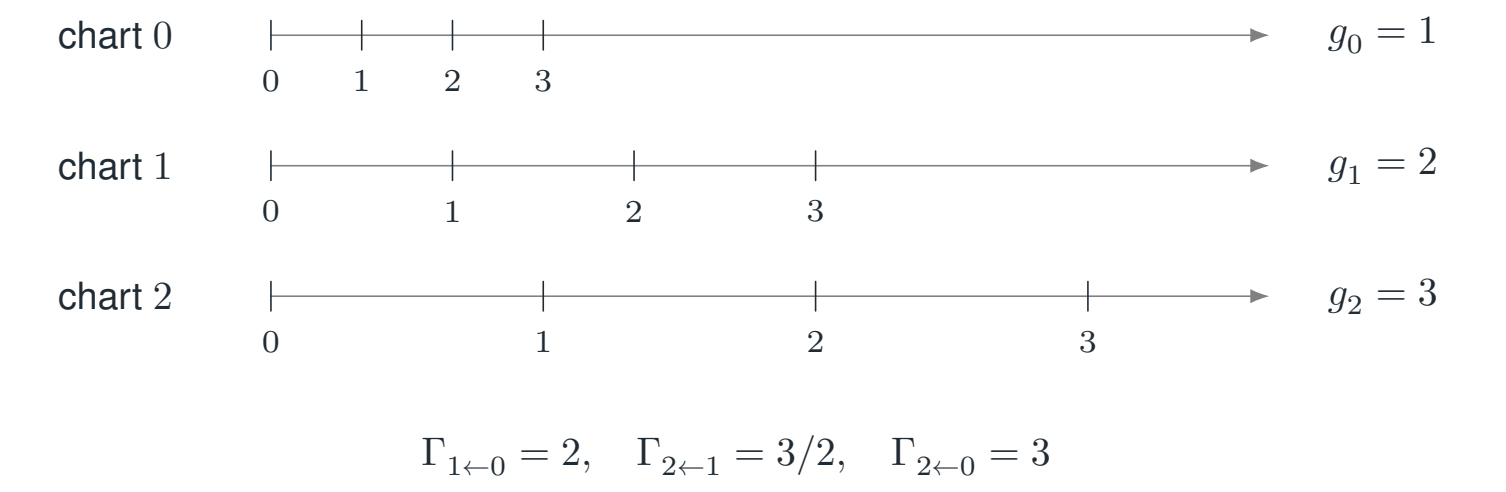
Reading the drawing
The rulers show marks scaled by the supplied gauge factors. Relative transports are ratios of target and source scales; the marks do not define an intrinsic metric.
Drawing labels and data 19 labels
Read the original labels as selectable text. Tables preserve grid relationships; other short labels are grouped compactly.
- chart \(0\)
- \(0\)
- \(1\)
- \(2\)
- \(3\)
- \(g_0=1\)
- chart \(1\)
- \(0\)
- \(1\)
- \(2\)
- \(3\)
- \(g_1=2\)
- chart \(2\)
- \(0\)
- \(1\)
- \(2\)
- \(3\)
- \(g_2=3\)
Evidence note from the source edition
The rulers display the chosen gauge scales: the marks are \(g_a n\) for integer \(n\). They visualize the supplied scalar factors, not an intrinsic metric. Relative transport is the ratio of the target and source scales.
The route through two steps \(0\to1\to2\) has multiplier \((3/2)2=3\), equal to the direct route \(0\to2\). More generally,
for every triple. Thus this connection is flat and reversible, but it is not calibrated to the original \(J\), whose values are identities.
Recovering the gauge from one root
Choose a base chart \(o\). The theorem constructs
With \(o=0\) and \(J=1\), the recovered \(G_a\) are exactly \(1,2,3\). The statement concerns the complete pairwise interface and its cocycle. It is not a topological claim about an arbitrary graph with missing direct comparisons.
Read this as
Flatness makes the chosen transports independent of path. Calibration identifies them with one particular canonical transport before any gauge change.