
Compare the linear equations \(F(x)=3x=0\) and \(G_A(x)=3x+3^A=0\), where \(A\ge2\). Their coefficient difference has \(3\)-adic valuation \(A\), but their roots differ by
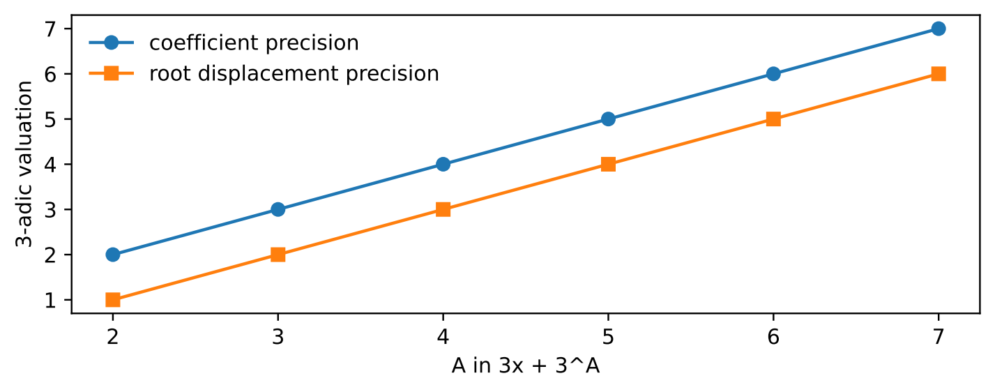
Reading the figure
For the displayed exponents two through seven, coefficient precision is the exponent, while root displacement precision is one less. Both lines rise with slope one. The derivative has valuation one, and the source derives the loss exactly from the two linear equations.
| Exponent | Root | Coefficient valuation | Displacement valuation |
|---|---|---|---|
| 2 | -3 | 2 | 1 |
| 3 | -9 | 3 | 2 |
| 4 | -27 | 4 | 3 |
| 5 | -81 | 5 | 4 |
| 6 | -243 | 6 | 5 |
| 7 | -729 | 7 | 6 |
Selectable labels from the original PDF
Native PDF text retains the figure’s extraction order. Equations and data tables above provide the reading order.
2
3
4
5
6
7
A in 3x + 3^A
1234567
3-adic valuation
coefficient precision
root displacement precision
The derivative has valuation one. Solving the correction equation divides by three, so one digit of coefficient precision is lost in root displacement. The calculation is exact for every displayed \(A\) and also follows immediately from the two linear equations.
This example explains why weighted lifting and deformation estimates track a Jacobian loss rather than silently treating every invertible derivative over \(\mathbb Q_p\) as a unit over \(\mathbb Z_p\). A valuation-zero derivative would not incur this particular loss. Nonlinear systems additionally require their stated neighborhood, residual, and right-inverse hypotheses.
Reproducibility. The eight examples use exact rational and integer arithmetic in tools/worked_examples.py. The release record states the executed finite ranges. This atlas adds no Lean endpoint and changes no formal claim in the companion.